Dealing with missing data is one of those fundamental challenges you hit early and often. It's not just about filling in blank cells; it's about making a deliberate choice. You can't just ignore the gaps, because doing so is an active decision that can seriously mess with your analysis. A good strategy is all about preserving the integrity of your dataset and making sure the models you build are accurate and reliable.

Why Your Missing Data Strategy Matters

Every empty cell in your dataset is a clue, and if you don't pay attention, you're bound to draw the wrong conclusions. These gaps aren't just a minor headache; they're potential sources of major bias that can completely invalidate your results. Honestly, knowing how to handle missing data is just as critical as picking the right algorithm for your model.

The reasons for these gaps are all over the place and really depend on where your data is coming from.

• Sensor Malfunctions: I've seen this a ton with IoT data. A sensor just gives out and stops recording temperature readings for a few hours.
• Survey Non-responses: This is a classic. Someone filling out a marketing survey decides they'd rather not share their income, so they just skip the question.
• Data Entry Errors: Good old-fashioned human error. Someone is manually typing in data and simply leaves a field blank by mistake.

Each of these scenarios introduces a different kind of risk. A faulty sensor might leave random gaps, which is one type of problem. But someone intentionally skipping a question introduces a systematic bias that could totally skew your model's understanding of user behavior. This is exactly why a one-size-fits-all approach is doomed to fail.

The Real-World Impact of Poor Data Handling

The consequences of getting this wrong go way beyond just a flawed model in a Jupyter notebook. Take financial markets, for example. Gaps in data are a constant battle due to market holidays, errors from data providers, or just different trading calendars across global exchanges. If you handle this missing financial data poorly, you could end up with faulty trading signals and tank an entire investment strategy. The economic stakes are incredibly high.

A smart missing data strategy is a huge piece of the puzzle when it to comes to addressing key data quality issues in general. It's not just about patching holes; it's about maintaining the credibility of your entire analytical pipeline.

Ultimately, your approach to missing data is a core part of your overall data hygiene. We've talked before about https://datanizant.com/data-cleaning-best-practices/, and building a solid missing data strategy is the logical next step. A thoughtful plan ensures whatever you build rests on a trustworthy foundation.

Diagnosing Your Missing Data Patterns

Before you can even think about fixing missing data, you need to put on your detective hat. Just running a quick .isnull().sum() gives you a raw count, but it doesn't tell you the story behind those gaps. To really get a handle on your dataset, you have to diagnose the patterns of missingness. The why is what dictates the how.

It’s tempting to just drop the rows with missing values and move on, but that's a classic rookie mistake. In fact, a recent review of 62 academic papers found that a staggering 72.6% of studies used listwise deletion—a technique that’s only appropriate for one specific type of missing data. This just goes to show how easy it is to pick the wrong tool for the job if you don't understand the underlying problem.

The Three Patterns of Missing Data

Getting to the root of your missing data is the single most important diagnostic step. There are three main patterns, and figuring out which one you're dealing with will shape your entire strategy.

• Missing Completely at Random (MCAR): This is the dream scenario, but it's also the rarest. Here, the missing data has absolutely no relationship with any other values, whether they're observed or missing. Imagine a sensor that occasionally fails because of a random hardware glitch—the missing temperature readings have nothing to do with the actual temperature outside.

• Missing at Random (MAR): This one's a bit more common. The missingness is related to some other observed data in your dataset, but not the missing value itself. For example, in a survey, men might be less likely to answer questions about their mental health. The missingness depends on the 'gender' column (which you have), not on the actual mental health score itself.

• Missing Not at Random (MNAR): This is the trickiest pattern to handle. The reason a value is missing is directly related to the value itself. The textbook example is a survey where high-income individuals are less likely to disclose their income. The very act of having a high income makes the data point more likely to be missing.

This isn't just academic hair-splitting; the distinction has massive implications. If you treat MNAR data as if it were MCAR, you can introduce serious bias into your analysis. Your model could end up learning the wrong patterns and making completely unreliable predictions.

If you want a refresher on the principles behind this, our guide on basic statistics concepts is a great place to start.

Visualizing these patterns is also a huge help. Python libraries like missingno can generate matrix plots that show you exactly where the gaps are in your dataframe. This gives you a bird's-eye view, making it much easier to spot potential correlations between missing values in different columns. This kind of visual diagnosis is a powerful first step toward choosing a fix that actually works.

When to Use Deletion Methods

Sometimes the simplest solution is the best one. When you're facing missing data, deletion is as straightforward as it gets. But don't let that simplicity fool you—using it in the wrong situation is one of the fastest ways to derail an otherwise solid analysis.

The real trick is knowing precisely when it’s safe to just drop the data.

Deletion methods, which mean removing either rows (listwise deletion) or entire columns (pairwise deletion), should only be on your radar under very specific circumstances. First and foremost, the data absolutely must be Missing Completely at Random (MCAR). If the reason a value is missing is tied to any other data point, observed or not, deleting it will inject bias into your results.

The second condition is all about quantity. The amount of missing data should be tiny. While there's no universal magic number, a good rule of thumb is that deletion is probably okay if less than 5% of your data is missing. Push past that, and you start running a serious risk of losing statistical power.

Listwise Deletion in Practice

Listwise deletion is the most common approach: you just remove any row that has a missing value. It’s dead simple to implement, but it’s also the most aggressive option.

Actionable Insight: Let's say you're working with a customer dataset of 10,000 rows. If 400 of those rows are missing a value for a single, non-critical feature like Last_Login_Date, and you've confirmed the missingness is random, dropping them might be a reasonable trade-off to get a perfectly clean dataset for a model that doesn't rely on that feature.

In Pandas, this is a one-liner:

# Drops any row that contains at least one missing value
clean_df = df.dropna()

That one command shrinks your DataFrame down, leaving you with only complete records. But think about this: if those 400 missing values were scattered across 400 different rows, you just threw out 4% of your entire dataset. That kind of reduction can weaken everything from your model's performance to the validity of your conclusions.

If you want a deeper dive into how sample size affects your analysis, check out our guide on statistical significance and confidence intervals.

The Risks of Deleting Columns

Wiping out an entire column is an even more drastic move. This is usually reserved for features where the data is so sparse that the column is practically useless for your analysis anyway.

Actionable Insight: If a customer_referral_code column is empty for 90% of your users, it probably doesn't hold much predictive power and could be dropped without much thought. Keeping it would likely just add noise to your model.

You can automate this by setting a threshold in Pandas:

# Drops columns that have less than 80% non-null values
df_cleaned_cols = df.dropna(axis='columns', thresh=len(df) * 0.8)

The Bottom Line: Use deletion methods with extreme caution. They're only safe when you're confident the data is MCAR and the amount you're losing is negligible. Making deletion your default move without a proper diagnosis is a shortcut that almost always leads to biased, unreliable results.

A Guide to Simple Imputation Techniques

When you can't afford to just delete rows with missing data—and let's be honest, that's most of the time—imputation is your next best friend. It’s the art of intelligently filling in the blanks. The simplest techniques are often the best place to start, especially when you're building a baseline model or just need to get a feel for your dataset.

These foundational methods are quick, straightforward to implement, and get you a complete dataset without much fuss. They usually involve replacing nulls with a single statistical value calculated from the rest of the column.

This visual shows just how much of an impact different imputation strategies can have on your model's performance.

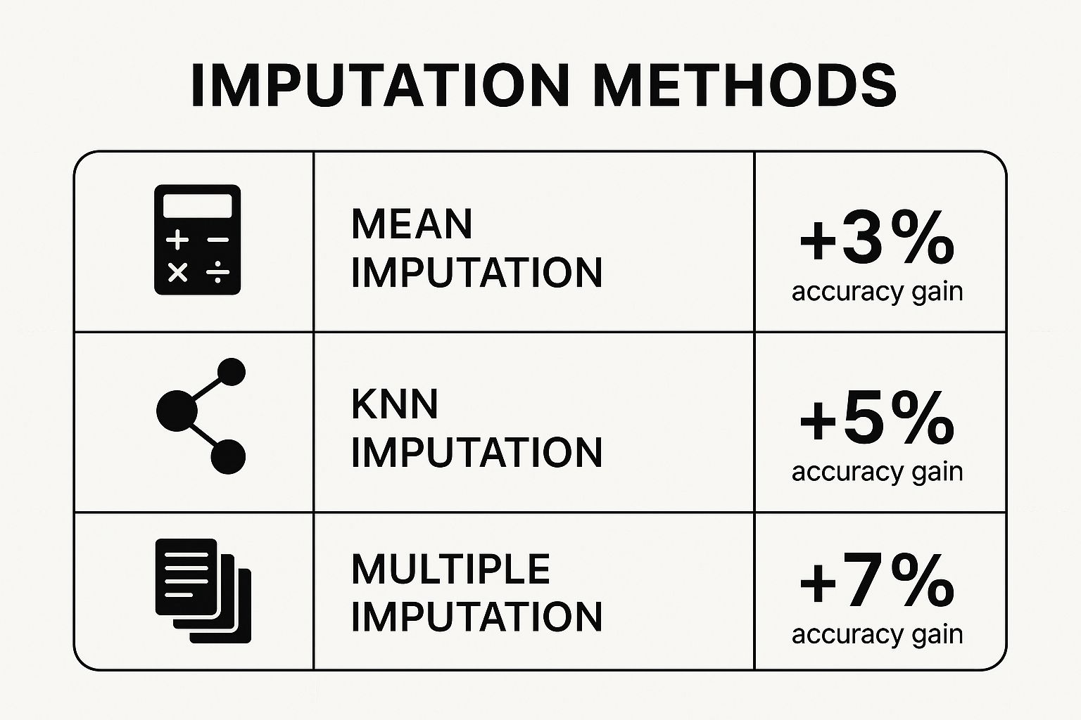
As you can see, even the most basic imputation gives you a leg up over doing nothing. However, it's also clear that more sophisticated approaches often deliver a bigger boost in accuracy.

Mean, Median, and Mode Imputation

Deciding between the mean, median, or mode isn't a coin toss. The right choice depends entirely on the shape and type of your data. Each one shines in a different scenario.

• Mean Imputation: This is your go-to for numerical data that's nicely bell-shaped (normally distributed) and free of crazy outliers. You simply plug in the column's average.
• Median Imputation: Got skewed numerical data or some extreme outliers? The median is your savior. It's the middle value, so it isn't yanked around by a few unusually high or low numbers.
• Mode Imputation: This one is strictly for categorical (non-numeric) data. It fills in the blanks with whatever value shows up most often in that column. Easy.

Actionable Insight: If you're working with a Household_Income column, using the mean would be a disaster. A handful of billionaires would drag the average way up, making your imputed values completely unrealistic for most households. The median, on the other hand, gives you a much more grounded, typical value.

Practical Application with Scikit-learn

Putting these ideas into practice is a breeze with Scikit-learn's SimpleImputer. It’s a clean, efficient tool for applying these strategies consistently.

Let’s imagine you need to fill in some missing Age values in your dataset using the median. Here’s how you’d do it:

from sklearn.impute import SimpleImputer
import numpy as np

# Create an imputer object with a median strategy
imputer = SimpleImputer(strategy='median')

# Reshape data and apply the imputer
age_column = df[['Age']].values
df['Age'] = imputer.fit_transform(age_column)

The beauty of this approach is that it prevents data leakage. The imputer object "learns" the median from your training data and can then apply that exact same value to any new data you feed it later on. For more hands-on code snippets, check out our complete guide on data cleaning in Python.

To help you decide which method is right for your situation, here's a quick comparison table summarizing the pros and cons of each.

Comparison of Simple Imputation Methods

Imputation Method	Best For	Main Advantage	Key Disadvantage
Mean Imputation	Normally distributed numerical data without outliers.	Very fast and easy to understand.	Highly sensitive to outliers and skewed data.
Median Imputation	Skewed numerical data or data with outliers.	Robust against extreme values.	Can distort the original data distribution.
Mode Imputation	Categorical (non-numeric) features.	Simple and effective for non-numeric data.	Can create an imbalance if one category dominates.

While these simple methods are a great starting point, they all share a common flaw: they can distort your data's natural variance and relationships.

A Critical Warning: Simple imputation techniques are popular for their efficiency, but they come with a major catch. They artificially reduce the natural variance in your data and can weaken the correlations between variables. Studies show these methods can introduce systematic errors, especially when more than 10% of the data is missing, potentially leading to unreliable conclusions.

Using Advanced Imputation for Better Accuracy

When simple fixes like mean or median imputation just won't cut it, it’s time to pull out the more advanced strategies. Sure, plugging a single number into a gap is quick, but it often completely misses the complex relationships between your features. This can weaken your model's predictive power. Advanced imputation techniques are built to preserve these intricate connections, giving you a much more solid foundation for your analysis.

These methods don't just look at one column in isolation. Instead, they use other features in the dataset to make a much more intelligent guess about what the missing value should be. By considering the full context of each data point, they generate realistic and nuanced values that better reflect how your data is actually distributed.

K-Nearest Neighbors (KNN) Imputation

One of the most intuitive and effective advanced methods is K-Nearest Neighbors (KNN) Imputation. The idea behind it is refreshingly simple: to fill a missing value, find the ‘k’ most similar complete data points (its "neighbors") and use their values to make an educated guess. For a numerical feature, this might mean taking the average of the neighbors' values. For a categorical one, you’d likely use the mode.

Actionable Insight: Think of it like trying to predict how someone would rate a new sci-fi movie. If you don't know their opinion, you could find five other people with nearly identical movie tastes (their nearest neighbors) and just average their ratings. This approach is almost always going to be more accurate than just using the average rating from all users.

Here’s how you can get this running with Scikit-learn:

from sklearn.impute import KNNImputer
import pandas as pd
import numpy as np

# Sample data with missing Age
data = {'Age': [25, 30, np.nan, 45, 22],
        'Salary': [50000, 60000, 75000, 90000, 48000]}
df = pd.DataFrame(data)

# Create a KNN imputer (let's use k=2 neighbors)
knn_imputer = KNNImputer(n_neighbors=2)

# Impute the missing values
df_imputed = pd.DataFrame(knn_imputer.fit_transform(df), columns=df.columns)

print(df_imputed)

In this snippet, the imputer finds the two data points that are most similar to the one with the missing age, using the Salary feature as a guide. It then uses their ages to calculate the new imputed value.

Model-Based Imputation with IterativeImputer

If you need even more power, you can turn to model-based imputation. Instead of just looking at neighbors, these techniques actually build a machine learning model specifically to predict the missing values. Scikit-learn's IterativeImputer is a fantastic tool for this job.

This imputer treats each feature with missing values as a target variable (y) and uses all the other features as its predictors (X). It then trains a regression model to predict the missing values. It's called "iterative" because it cycles through each feature, updating its predictions over and over until the imputed values stop changing much.

By modeling each feature as a function of the others, IterativeImputer can uncover complex, nonlinear relationships that simpler methods would miss entirely. This makes it an excellent choice for datasets where features are highly correlated.

The process is definitely more computationally intensive, but the payoff in accuracy is often well worth it. It’s become a key part of the modern toolkit for effective data preprocessing in machine learning, ensuring your dataset is as complete and reliable as possible before you even think about training your final model.

Let's see it in action:

from sklearn.experimental import enable_iterative_imputer
from sklearn.impute import IterativeImputer

# Sample data from the previous example
data = {'Age': [25, 30, np.nan, 45, 22],
        'Salary': [50000, 60000, 75000, 90000, 48000]}
df = pd.DataFrame(data)

# Create an IterativeImputer instance
iterative_imputer = IterativeImputer(max_iter=10, random_state=0)

# Apply the imputer
df_iterative_imputed = pd.DataFrame(iterative_imputer.fit_transform(df), columns=df.columns)

print(df_iterative_imputed)

Choosing an advanced method like KNN or IterativeImputer is a strategic call. It'll demand more from your machine, but it pays you back with better model performance, especially when preserving the true underlying structure of your data is critical.

Frequently Asked Questions

Even after you've built a solid strategy, you'll inevitably run into specific questions mid-project. Knowing how to handle missing data is all about having quick, clear answers for these common hurdles. Let's dig into some of the questions that pop up most often.

What Percentage of Missing Data Is Acceptable to Delete?

This is the classic question, but there's no magic number. You'll often hear a rule of thumb that if less than 5% of the data is missing, you might be okay just deleting those records. But—and this is a big but—that only holds if you're confident the data is Missing Completely at Random (MCAR).

Context is everything here. If you're working with a massive dataset of a million records, dropping 5% probably won't hurt your statistical power. But in a small dataset of 200 records, that same 5% could be a huge loss of valuable information.

Actionable Insight: Before you even think about deleting, you have to consider the potential for bias. If the reason a value is missing is related to another variable in your dataset (e.g., people with lower income are less likely to report it), deletion—even a tiny amount—can seriously skew your results. I almost always lean towards imputation over deletion to be safe.

How Do I Choose Between Mean, Median, and Mode Imputation?

The right choice comes down to your data's type and its distribution. This isn't a one-size-fits-all situation, and grabbing the wrong one will distort your dataset.

Here’s my mental checklist for this:

• Use Mean Imputation for numerical data that follows a nice, clean normal distribution (a bell curve) and doesn't have any wild outliers. The average is a perfectly good stand-in here.
• Use Median Imputation for numerical data that's skewed or has outliers. The median is much more resilient to extreme values, giving you a far more representative number.
• Use Mode Imputation for categorical (non-numeric) features. You can't average categories like "red," "blue," and "green," so filling in the most common value is the logical move.

Practical Example: If you're filling in a missing household_income value and your dataset includes a few billionaires, using the mean would be a huge mistake. Their incomes would drag the average way up. The median, on the other hand, would give you a much more realistic value for a typical household.

Can Machine Learning Models Handle Missing Data Automatically?

Some of the more modern algorithms, like LightGBM and XGBoost, are pretty smart about this. They're designed to handle missing values internally, essentially learning which path to take at a decision tree split when a value isn't there.

However, most of the classic models—think Linear Regression, Logistic Regression, or Support Vector Machines (SVMs)—will just stop and throw an error. They can't process NaNs at all, so you absolutely have to preprocess your data for them.

Actionable Insight: Even when I'm using a model that can handle NaNs, I still make it a habit to handle missing data explicitly myself. It gives you total control over the data pipeline, keeps things consistent if you decide to try a different model later, and you know exactly how those gaps were filled. As we covered in our guide to data preprocessing for machine learning, taking control of this step is fundamental to building models you can actually trust.

---

At DATA-NIZANT, we provide expert-authored articles to help you navigate complex topics in AI, machine learning, and data science. Stay ahead of the curve by exploring our in-depth analyses and practical guides at https://www.datanizant.com.