
Data cleaning in Python is the process of finding and fixing all the inevitable errors, inconsistencies, and plain weirdness in a dataset. Think of it like a chef prepping ingredients before a big service. If you don't wash the vegetables or trim the fat, the final dish—your analysis or machine learning model—is going to be disappointing, or even inedible.
The main jobs here involve tackling missing values, tossing out duplicate records, standardizing messy formats, and dealing with those oddball outliers, all primarily using the workhorse library, Pandas.
Why Data Cleaning Is Your Most Critical First Step
Look, before you can dream of building a fancy predictive model or a stunning dashboard, you have to be able to trust your data. Data cleaning in Python isn't just a box-ticking exercise; it's the strategic foundation that ensures your entire project is sound. Rushing this part is like building a house on a swamp. It will collapse.
Dirty data is a silent killer for projects. A simple duplicated row can make your customer count look twice as big, leading to wildly optimistic sales reports. A number accidentally stored as text can crash your entire analysis script. These aren't just hypotheticals—they're the daily headaches of anyone working with data. The goal is to systematically hunt down and fix these problems, turning a chaotic, unreliable spreadsheet into a clean, trustworthy asset.
The Real Cost of Neglecting Data Quality
Skipping over proper data cleaning isn't just a technical mistake; it's a financial one. All that time you spend scratching your head over bizarre results or re-running failed analyses? It almost always traces back to a data issue that could have been fixed from the start.
In fact, most industry experts agree that data cleaning eats up a staggering 60-80% of the total time on any given data science project. That number alone should tell you how pivotal this phase is. The quality of your output is directly tied to the quality of your input.
"Garbage in, garbage out" is the oldest cliché in data science for a reason. No amount of advanced modeling or sophisticated algorithms can compensate for poor-quality data. Your model is only as good as the data it's trained on.
Common Data Impurities and Their Real-World Impact
To make this less abstract, let’s look at the specific gremlins that hide in datasets and the real-world chaos they cause. Understanding these direct consequences helps you see cleaning not as a chore, but as essential risk management. If you want to get ahead of these issues, our guide on data cleaning best practices provides a more structured framework.
The following table breaks down the usual suspects and illustrates the very real damage they can do if you let them slide.
Common Data Impurities and Their Real-World Impact
| Data Issue | Example Scenario | Impact if Ignored |
|---|---|---|
| Duplicate Records | A customer appears twice in a sales database due to a typo during data entry. | Skewed summary statistics, such as inflated customer counts and inaccurate average revenue per user. |
| Missing Values | A survey dataset is missing the age for 20% of respondents. |
Reduced sample size if rows are dropped, or biased results if filled improperly. |
| Incorrect Data Types | Product prices are stored as text strings (e.g., "$19.99") instead of numbers. | Inability to perform mathematical calculations like summing total sales or finding the average price. |
| Inconsistent Formatting | A State column contains "CA", "ca", and "California". |
Groups and filters will fail to capture all relevant data, leading to incomplete analysis. |
| Outliers | A single data entry error shows a product sold for $1,000,000 instead of $10.00. | Drastically skewed averages and other statistical measures, leading to poor model performance. |
Each of these issues can single-handedly invalidate your findings. By methodically addressing them with Python and Pandas, you're not just cleaning—you're building a foundation of trust that ensures every subsequent step, from exploration to modeling, stands on solid ground.
Strategies for Handling Missing Data in Pandas

Missing data isn't just an annoyance; it's a fundamental challenge you'll face in almost every real-world dataset. The choices you make to handle these gaps directly impact the credibility of your analysis and the performance of your models.
It’s tempting to just remove any row or column with a missing value, but that's a blunt approach that can easily throw away valuable information. A thoughtful strategy for data cleaning in python requires a bit more nuance.
The first call you often have to make is whether to drop rows or entire columns. If a column is mostly empty and not critical to your analysis, dropping it with df.drop(columns=['column_name']) is a clean, decisive move. But what if the column is important and just a few rows have missing values, say less than 5%? In that case, dropping those specific rows with df.dropna() is often a reasonable trade-off.
When to Remove vs. When to Impute
Deciding whether to drop data or fill it in (a process called imputation) is a critical judgment call. Dropping data is the easy path, but it shrinks your dataset. Imputation, on the other hand, preserves your data but introduces assumptions that you need to be comfortable with.
Here’s an actionable insight for making this choice:
- How much data is missing? If a column is missing over 60-70% of its values, any information you impute would be more made-up than real. In those situations, dropping the column is usually the safest bet.
- How important is the feature? If the column is a key predictor for your machine learning model or central to your business question, you should try everything you can to impute the values rather than lose the feature entirely.
- What kind of data is it? The right imputation strategy depends heavily on whether your data is numerical or categorical and how it's distributed.
Making these decisions is a core part of the analytical process. It's where the art of data science meets the science, and it ties directly into the project's larger goals. As covered in our guide on data science project management, your cleaning choices must align with your ultimate analytical objectives.
Practical Imputation Techniques in Pandas
Once you've decided to fill in missing values, pandas gives you some powerful and straightforward methods. The most common techniques involve filling NaN values with a statistical measure from the column itself.
Let's imagine we have a dataset of house sales with a square_footage column that has some missing entries.
1. Filling with the Mean
The mean is a solid default choice for numerical data that follows a normal (bell-curve) distribution.
Practical Example:
# Calculate the mean of the column
mean_sqft = df['square_footage'].mean()

# Fill missing values with the mean
df['square_footage'].fillna(mean_sqft, inplace=True)
But be careful—the mean is very sensitive to outliers. If your dataset includes a few massive mansions, the mean square_footage could be pulled artificially high, making it a poor representation for a typical home.
2. Filling with the Median
The median is the middle value in a sorted list, which makes it resistant to outliers. This is a much safer choice for skewed data, which is common with things like income or house prices.
Practical Example:
# Calculate the median
median_sqft = df['square_footage'].median()

# Fill missing values with the more robust median
df['square_footage'].fillna(median_sqft, inplace=True)
Using the median here provides a much more realistic value, preventing a few extreme data points from skewing the data you're filling in.
Pro Tip: Always visualize your data's distribution before choosing between the mean and median. A quick histogram with
df['column'].hist()can save you from making a biased choice that harms your analysis later on.
3. Filling with the Mode
For categorical data, like a neighborhood column, you can't calculate a mean or median. In this scenario, the mode—the most frequently occurring value—is the logical choice.
Practical Example:
# Find the most common category
mode_neighborhood = df['neighborhood'].mode()[0]

# Fill missing categorical data with the mode
df['neighborhood'].fillna(mode_neighborhood, inplace=True)
Advanced Filling Strategies
Sometimes, simple statistical fixes aren't enough. For time-series data, where observations are ordered chronologically, using the last known value is often a more logical approach. The forward-fill method (ffill) is perfect for this.
Practical Example:
# Forward-fill missing stock prices from the previous day
df['stock_price'].fillna(method='ffill', inplace=True)
This method assumes the value simply hasn't changed since the last observation, a common and often safe assumption in sensor readings or financial data. The opposite is backward-fill (bfill), which uses the next known value. These contextual methods show how a deeper understanding of your data can lead to much smarter and more accurate cleaning decisions.
Finding and Removing Duplicates with Precision

Once you’ve dealt with missing values, the next big task is hunting down duplicate records. These are the sneakiest troublemakers in a dataset. They won’t crash your script or throw obvious errors, but they'll quietly inflate counts, skew averages, and completely undermine your analysis.
Think about it: a sales report where one big transaction gets recorded three times. Your revenue for the week suddenly looks incredible, but it's a house of cards. Thankfully, pandas gives us a simple, powerful way to find and root out these deceptive entries.
How to Spot Duplicates in Your Dataset
First things first, you need to see if you even have a duplicate problem. The df.duplicated() method is perfect for this initial check. It scans your DataFrame and returns a Boolean Series—True for any row that's an exact copy of one that came before it, and False otherwise.
Practical Example:
# Count the total number of duplicate rows
total_duplicates = df.duplicated().sum()
print(f"Found {total_duplicates} duplicate rows.")
This one-liner gives you an immediate sense of the scale of the problem. If that number is high, you know right away that your summary stats, like customer counts or total sales, are probably wrong.
A Practical Example of Removing Duplicates
After you've identified them, getting rid of duplicates is usually as simple as calling df.drop_duplicates(). By default, this function keeps the first instance of a duplicated row and gets rid of the rest.
But what if you need more control? Let's imagine a customer list where people might have signed up more than once.
| customer_id | signup_date | |
|---|---|---|
| 101 | anna@email.com | 2023-01-15 |
| 102 | ben@email.com | 2023-02-10 |
| 101 | anna@email.com | 2023-03-20 |
| 103 | carla@email.com | 2023-04-05 |
Here, customer 101 shows up twice. An actionable insight is to define a business rule for which record to keep. In this case, we'll keep their most recent record.
Practical Example:
# First, sort by date so the newest record is last
df_sorted = df.sort_values('signup_date')

# Now, drop duplicates on 'customer_id', keeping the 'last' entry
df_cleaned = df_sorted.drop_duplicates(subset=['customer_id'], keep='last')
This is much more intelligent than a blanket removal. It lets you define what a "duplicate" actually means for your project—in this case, it’s a shared customer_id—and apply business logic to decide what to save.
A Critical Workflow Insight: Always remove duplicates before you start filling in missing values. If you impute first, you might waste time filling NaNs in a row that gets dropped seconds later. Worse, your imputation logic (like a column mean) could be based on an inflated, incorrect dataset.
A typical data cleaning workflow in Python starts by dropping duplicate rows. This is a foundational step because duplicate data can seriously skew your results, from simple averages to complex model predictions. For example, if you remove duplicates first, any subsequent median calculations you use to fill in missing numbers will be accurate. This sequence ensures every calculation you perform is on a clean, unique set of records. This principle is a cornerstone of effective data preprocessing for machine learning, where the order of your cleaning steps can make or break your model's performance. By tackling duplicates first, you safeguard the integrity of your entire cleaning process.
Standardizing Formats and Correcting Data Types
After you've dealt with missing values and duplicates, your dataset is looking much cleaner. But don't pop the champagne just yet. Some of the most frustrating errors are the subtle ones, like inconsistent formatting and incorrect data types, which can silently sabotage your analysis or crash your scripts entirely.
These issues often hide in plain sight. For example, your program will see "USA," "usa," and "United States" as three completely different categories. Or a price column might be stored as text (an object type in pandas) just because of a single dollar sign, making any math impossible. Data cleaning in Python isn't finished until every column is standardized and machine-readable.
Fixing these problems is all about enforcing consistency. It’s the only way to guarantee that when you group, filter, or run calculations, you're working with data that behaves exactly as you expect. Thankfully, pandas has just the tools for these jobs.
Normalizing Text and Categorical Data
Inconsistent capitalization is a classic data quality headache. For any text-based categorical column, a simple but powerful first step is to convert everything to a single case—usually lowercase. This one move stops your code from treating "Apple" and "apple" as two distinct items.
The .str.lower() method in pandas is your best friend here. Let's say we have a product_category column that's a total mess of mixed cases.
Practical Example:
# A sample of our messy 'product_category' column
# 0      Electronics
# 1    home & garden
# 2      electronics
# 3           Toys
# 4    Home & Garden

# Standardize the column to all lowercase
df['product_category'] = df['product_category'].str.lower()

# Now the column is clean and consistent
# 0      electronics
# 1    home & garden
# 2      electronics
# 3           toys
# 4    home & garden
It seems minor, but this change makes your groupby() operations and value counts accurate. It’s a foundational step for any reliable analysis of categorical data.
Converting to Proper Data Types
I can't count how many times I've seen analyses fail because of columns stored with the wrong data type. A sales_amount column stuck as a string (object) because of currency symbols or commas will throw a TypeError the second you try to find its sum.
The .astype() method is the workhorse for type conversion. But here's the catch: you almost always have to clean the string data first before you can convert it.
Practical Example:
# Our 'price' column is stored as text with '$' and ','
# 0    $1,200.50
# 1       $50.00
# 2      $999.99
# Name: price, dtype: object

# First, remove the non-numeric characters using .str.replace()
df['price'] = df['price'].str.replace('$', '', regex=False).str.replace(',', '', regex=False)

# Now, convert the cleaned string column to a float
df['price'] = df['price'].astype(float)

# The column is now a numeric type, ready for calculation
# 0    1200.50
# 1      50.00
# 2     999.99
# Name: price, dtype: float64
This two-step pattern—clean then convert—is an actionable insight you’ll use over and over again.
Key Takeaway: Correcting data types isn't just about preventing errors. It dramatically improves memory usage and computational speed, since numeric types are far more efficient for pandas to process than generic
objecttypes. This becomes a game-changer when you start working with larger datasets.
Handling Dates and Times with Precision
Dates are notoriously tricky. They show up in all sorts of formats—"01-25-2023", "Jan 25, 2023", "2023/01/25"—which are just meaningless strings to a computer. To do any kind of time-based analysis, you absolutely must convert them into a standard datetime object.
Pandas' pd.to_datetime() function is a lifesaver here. It’s smart enough to parse most common date formats on its own, without you having to spell out the format.
Practical Example:
# Our 'order_date' column has inconsistent formats
# 0    2023-03-15
# 1    04/10/2023
# 2    May 5, 2023
# Name: order_date, dtype: object

# Convert the column to a proper datetime format
df['order_date'] = pd.to_datetime(df['order_date'])

# The column is now a standardized datetime object
# 0   2023-03-15
# 1   2023-04-10
# 2   2023-05-05
# Name: order_date, dtype: datetime64[ns]
Once converted, you can easily pull out the year, month, or day of the week, opening the door to powerful time-series analysis. These clean formats are also a non-negotiable prerequisite for accurate inputs. As detailed in our overview of machine learning model monitoring, this kind of data quality work directly impacts model performance down the line.
With your data formats now clean and consistent, it's time to go on a hunt for outliers. These are the oddball data points that sit way outside the norm, and they can be incredibly deceptive.
Think about it: a simple typo creating an impossibly high price, or a sensor glitch logging a negative age. A single one of these anomalies can throw off your entire analysis, skewing statistical models and leading to terrible predictions. Good data cleaning in python isn't just about finding these troublemakers; it's about figuring out a smart way to handle them.
You can't just ignore outliers. They have the power to drag your mean up or down, inflate your standard deviation, and ultimately make your models a poor reflection of reality. The trick is to use solid statistical methods to flag them and then choose a strategy—which, by the way, doesn't always mean deleting them.
Finding Outliers with the Interquartile Range (IQR)
One of my go-to methods for finding outliers, especially when the data isn't perfectly bell-shaped (a situation we call "skewed"), is the Interquartile Range (IQR) method. The beauty of the IQR is that it focuses on the middle 50% of your data, so it's naturally resistant to being thrown off by extreme values.
The logic is pretty simple:
- Find the Quartiles: First, you calculate the first quartile (Q1), which marks the 25th percentile, and the third quartile (Q3), the 75th percentile.
- Calculate the IQR: Just subtract Q1 from Q3. This gives you the spread of the middle half of your data.
IQR = Q3 - Q1. - Set the Fences: Finally, you define the "fences" or boundaries. Anything that falls outside these is flagged as a potential outlier.
- Lower Fence:
Q1 - 1.5 * IQR - Upper Fence:
Q3 + 1.5 * IQR
- Lower Fence:
Here’s how that looks in practice. Let's say we're looking at a sale_price column in our DataFrame:
Practical Example:
import numpy as np

Q1 = df['sale_price'].quantile(0.25)
Q3 = df['sale_price'].quantile(0.75)
IQR = Q3 - Q1

lower_bound = Q1 - 1.5 * IQR
upper_bound = Q3 + 1.5 * IQR

# This will give you a new DataFrame with just the outliers
outliers = df[(df['sale_price'] < lower_bound) | (df['sale_price'] > upper_bound)]
print("Found outliers:")
print(outliers)
This snippet is great because it isolates the outlier rows, letting you take a closer look before you decide their fate.
Using Z-Scores for Normally Distributed Data
Now, if your data happens to follow a nice, clean normal distribution (the classic bell curve), the Z-score is a fantastic tool for the job. A Z-score simply tells you how many standard deviations away from the mean a particular data point is.
A common rule of thumb I've used for years is to treat any data point with a Z-score above 3 or below -3 as a potential outlier.
Practical Example:
from scipy import stats

# This adds a new 'z_score' column to your DataFrame
df['z_score'] = np.abs(stats.zscore(df['sale_price']))

# Now, filter for outliers using a Z-score threshold of 3
outliers = df[df['z_score'] > 3]
print("Found outliers:")
print(outliers)
The Z-score method is powerful, but a word of caution: only use it if you're fairly certain your data isn't heavily skewed. Why? Because the mean and standard deviation—the very building blocks of the Z-score—are themselves easily influenced by outliers. It can become a bit of a circular problem.
Choosing Your Outlier Detection Method
Picking the right method depends entirely on the shape of your data. The Z-score is fast and effective for symmetrical, bell-curved distributions, while the IQR method is much more robust and reliable for data that leans to one side.
Here’s a table to help you decide which tool to pull out of your toolbox.
| Method | Best For | Core Logic | Example Python Implementation |
|---|---|---|---|
| IQR Method | Skewed (non-normal) data | Identifies values outside 1.5x the interquartile range from the 1st/3rd quartiles. | Q1 = df['col'].quantile(0.25)Q3 = df['col'].quantile(0.75)IQR = Q3 - Q1 |
| Z-Score | Normally distributed data | Flags data points more than 3 standard deviations from the mean. | from scipy import statsdf['z_score'] = np.abs(stats.zscore(df['col'])) |
Ultimately, understanding your data's distribution is the first step to choosing a method that won't lead you astray.
This image gives a great high-level view of how you can visualize your data's problems and then use code to implement the fixes.
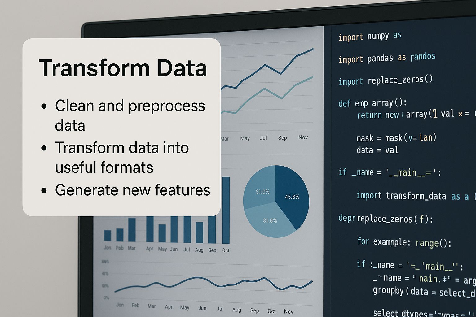
They're two sides of the same coin: seeing the problem with charts and fixing it with code is what effective data cleaning is all about.
So, What Do You Do with Outliers?
Okay, you've found an outlier. The hunt is over, but the work isn't. Your next move is critical.
-
Remove Them: This is the most drastic option. If you're absolutely sure an outlier is a mistake—like a data entry error logging a person's height as 10 feet—then deleting it is usually the safest bet.
-
Cap Them (Winsorizing): Instead of outright deletion, you can "cap" the outliers. This means you replace any value above your upper fence with the upper fence value itself (and do the same for the lower fence). This keeps the data point in your set but neutralizes its ability to skew the results.
-
Transform Them: For skewed data, sometimes a mathematical transformation is the answer. Applying a function like a logarithm (
np.log()) can help pull the long tail of a distribution in, making the outliers less extreme and the data easier to model.
Actionable Insight: Whatever you do, never blindly delete outliers. An outlier could be a genuine, if rare, data point. In fraud detection, for example, the outlier is often the exact thing you're looking for! Always stop and investigate the context before you act.
Getting these steps right is fundamental to building a data pipeline you can trust. This entire process mirrors the principles we talk about in our guide on mastering AI workflow automation, where having a logical, repeatable system for handling data is the key to success.
Of course. Here is the rewritten section, designed to sound like an experienced human expert and match the provided style examples.
Common Questions About Data Cleaning in Python
As you get your hands dirty with data cleaning in Python, you'll inevitably run into the same questions that trip up even seasoned pros. Getting comfortable with these common challenges is what separates a good data practitioner from a great one. Let's tackle some of the most frequent questions I see come up in real-world projects.
This is especially true now that so much data comes from automated sources. Python’s role in data cleaning has exploded with the rise of web scraping and other data collection tools. Why? Because scraped datasets are notoriously messy—they're often riddled with missing values, formatting errors, and duplicates that can completely throw off an analysis. It’s not uncommon for scraped data to have 5% to 20% duplicate rows, and I’ve seen missing values plague 10-30% of the columns. Knowing how to handle these issues is non-negotiable, and you can get a deeper sense of these web data challenges from Apify's analysis.
How Do I Decide Whether to Drop or Fill Missing Data?
The classic dilemma: to drop or to fill? The answer always depends on the amount and the context of what’s missing. There's no magic formula here; it's a strategic decision you have to make.
If a tiny fraction of your rows have missing values—say, under 5%—and your dataset is massive, dropping them is often the simplest path forward. It's clean, quick, and unlikely to skew your results. But what if a critical feature column is full of holes? Dropping it would mean throwing away potentially valuable predictive power.
An Actionable Insight: Always weigh the trade-off. Are you losing more by dropping entire records, or are you risking more by introducing potential bias from filling them in? For example, in a customer dataset, you'd probably try to impute a missing
ageto keep the customer's record. But if a row is missing acustomer_id, it's useless—you can't identify them, so you might as well drop it.
What Is the Best Library for Data Cleaning in Python?
Let’s be direct: for data cleaning in Python, pandas is the undisputed king. Its DataFrame structure is perfectly built for the kind of slicing, dicing, and transforming that cleaning demands. It gives you intuitive, powerful functions for nearly every task we've covered, from spotting duplicates and handling missing values to fixing data types.
While other libraries are important, they usually play a supporting role to pandas.
- NumPy: The workhorse that powers pandas under the hood. You'll lean on it for heavy-duty numerical computing and mathematical functions.
- scikit-learn: Comes into play when you need more advanced imputation methods for machine learning, like its
KNNImputerorIterativeImputer. - OpenRefine: While not a Python library, it’s a phenomenal standalone tool for wrestling with exceptionally messy data before you even think about bringing it into a Python environment.
Honestly, though, a solid 95% of your day-to-day cleaning work can be handled brilliantly with pandas alone. If you're going to master one thing, make it pandas.
Can I Automate My Data Cleaning Process?
Absolutely—in fact, you should. The real goal isn't just to clean a single file in a Jupyter Notebook. It's to build a reproducible data cleaning pipeline. This is where using a scripting language like Python really shines.
An actionable insight is to think of your cleaning process as a recipe that can be automated:
- Load the raw data.
- Fix column data types.
- Standardize text formatting.
- Remove duplicate records.
- Address missing values.
- Handle outliers.
- Save the clean, ready-to-use dataset.
This approach guarantees consistency every time you get a new batch of data. As we often stress in our Datanizant articles, like our piece on mastering AI workflow automation, this transforms a boring, manual chore into a scalable, automated asset. It saves a ton of time and, more importantly, prevents human error.
How Does Cleaning for ML Differ from General Analysis?
The core tasks are the same—you're still finding duplicates and handling NaNs. But when you're preparing data for machine learning, the mindset is far more rigid because of one critical concept: data leakage.
Data leakage happens when information from outside the training dataset sneaks its way into your model. If your model gets a peek at the test data during training, even by accident, its performance metrics will be artificially inflated. It'll look amazing on your screen but will completely fail when deployed in the real world.
Here's an actionable insight to avoid this:
- Split First: The absolute first thing you do is split your data into training and testing sets. No exceptions.
- Fit on Train Only: Any transformation that "learns" from the data—like an imputer calculating a mean or a scaler finding a min/max value—must be
fitonly on the training data. - Transform Both: You then apply that same fitted transformer to update both the training set and the test set.
This strict process, which is foundational to topics like data preprocessing for machine learning, ensures your model learns patterns exclusively from the training data, leaving the test set as a truly untouched benchmark. Missing this step is one of the most common and costly mistakes I see new practitioners make.
At DATA-NIZANT, we believe that clean data is the bedrock of all meaningful insights. Our articles are designed to give you the practical knowledge to turn messy, real-world data into a reliable asset. Explore more expert-authored guides and in-depth analyses at https://www.datanizant.com.

