Master Feature Engineering Techniques to Boost Model Accuracy

Think of your raw data as a pile of ingredients for a gourmet meal. You could have the most expensive, high-tech oven in the world (your algorithm), but if you just toss in unwashed, uncut, and unseasoned vegetables, the result will be… disappointing.

Feature engineering is the art of data preparation. It's the meticulous process of transforming those raw ingredients—your data—into something your machine learning model can truly work with. This isn't just about cleaning things up; it's about creatively and strategically shaping your data to highlight the patterns that matter most.

Why Feature Engineering Is Your Secret Weapon in AI

At its heart, feature engineering is about translating your real-world knowledge into a language a machine can understand. By creating new features or modifying existing ones, you make the underlying problem much clearer for your predictive models, making it far easier for them to learn and deliver accurate results.

Better features, not necessarily more complex algorithms, are what separate good models from great ones. It's often the most critical and time-consuming part of a project, but the payoff is enormous.

The Real-World Impact on Model Performance

The quality of your features directly sets the performance ceiling for your model. It’s a simple truth: a basic model fed with excellent features will almost always beat a complex, "state-of-the-art" model that's working with mediocre data.

Well-crafted features have a few major benefits:

• They Boost Accuracy: Good features make the relationship between your inputs and the target outcome more explicit and easier for the model to detect.
• They Simplify Your Models: Powerful features often mean you can use a simpler, faster, and more interpretable model. No need for a sledgehammer when a scalpel will do.
• They Build More Robust Systems: Models trained on strong, meaningful features tend to be more resilient when they encounter new, unseen data in the real world.

For example, giving a model a raw customer signup_date is okay, but it's not very direct. If you engineer a new feature like days_as_customer, you've created a much more powerful signal for predicting things like customer churn or lifetime value. It’s a simple change, but it speaks volumes.

Actionable Insight: The aim of feature engineering isn't just to tidy up your data—it's to enrich it. Think of it as giving your model helpful clues and context, guiding it toward a smarter, more reliable conclusion. For example, instead of using raw latitude and longitude to predict delivery times, create a new feature like distance_from_warehouse to give the model a direct, actionable signal.

To get a better sense of the different ways we can transform our data, let's look at the main categories of feature engineering.

Core Feature Engineering Categories at a Glance

This table gives a quick overview of the core techniques we'll be breaking down. Each one serves a different purpose in getting our data ready for a machine learning model.

Technique Category	Primary Goal	Practical Example
Imputation	Fill in missing or null values in the dataset.	Replacing a missing age value with the average age of all users.
Encoding	Convert categorical (non-numeric) data into a numerical format.	Turning a color column with "Red", "Green", "Blue" into [1,0,0], etc.
Scaling	Standardize the range of numerical features.	Rescaling income and age to be on a similar 0-to-1 scale.
Transformation	Modify the distribution of a feature to improve model stability.	Applying a log transformation to a skewed sales feature.
Feature Generation	Create new features from existing ones.	Calculating price_per_sq_ft from price and square_footage.
Feature Selection	Identify and remove irrelevant or redundant features.	Dropping features that have little to no correlation with the outcome.

Each of these categories contains a whole toolbox of methods, and knowing which one to use—and when—is a key skill for any data professional.

From Manual Craft to Automated Discovery

The idea of crafting features isn't new. The field took a major turn in the 1990s, shifting from purely knowledge-based systems to more data-driven approaches. With models like support-vector machines (SVMs) gaining popularity, the quality of the input data became more critical than ever.

More recently, the deep learning boom of the 2010s brought powerful techniques for automated feature discovery, especially for unstructured data like images and text. But even with these incredible advances, manual, domain-driven feature engineering is still essential. In fields like finance or healthcare, an expert's intuition is often the key to creating a truly predictive signal that an algorithm might miss on its own. If you're curious about the timeline, you can learn more about the history and evolution of machine learning.

Ultimately, getting comfortable with these feature engineering techniques is what gives you a real advantage. It’s what lets you step away from the default settings and start building AI that solves your specific problem with a level of precision and power you can't get otherwise.

Creating Powerful Features From Your Existing Data

Once your data is clean and organized, the real fun begins. This is where we get to the most creative part of feature engineering: crafting brand-new, high-impact features from the ones you already have. Think of it as transforming raw information into powerful signals that scream out the underlying patterns to your machine learning model.

These new features act like shortcuts. Instead of forcing the model to figure out complex relationships from scratch, you're essentially handing it the answers on a silver platter. It's often this step that separates a decent model from a truly exceptional one.

Uncovering Hidden Patterns With Interaction Features

One of the most effective ways to boost model performance is by creating interaction features. This is all about combining two or more features, usually with simple math like multiplication or division, to capture how they work together.

Actionable Insight: Always look for features that might have a synergistic effect. A model might struggle to learn that "high frequency" and "high value" together signal a top-tier customer. By creating an interaction feature, you explicitly state this relationship, making the model's job a whole lot easier.

Practical Example: Creating Interaction Features

Let's imagine we're working with a real estate dataset to predict housing prices. We have two basic features:

• number_of_rooms: The total room count in a house.
• square_footage: The total area of the house.

Sure, a bigger house with more rooms is usually more expensive. But what about the spaciousness of the house? A home with lots of tiny, cramped rooms is very different from one with fewer but larger, more open rooms.

We can capture this nuance by creating an interaction feature:

• New Feature: avg_room_size = square_footage / number_of_rooms

This new feature provides critical context that wasn't immediately obvious, helping the model make smarter distinctions between different types of properties.

Simplifying Complexity With Binning

Another fantastic method is binning, which is just a fancy term for grouping continuous numbers into discrete categories or "bins." This is incredibly useful for cutting through the noise of small data variations and capturing relationships that aren't perfectly linear.

Think about a customer churn model. You have a feature for account_tenure, measured in months. Is a customer who has been with you for 35 months fundamentally different from one at 36 months? Probably not. Treating every single month as a unique value can add more confusion than clarity.

By binning this data, you can group customers into more meaningful categories.

Practical Example: Binning a Customer Churn Dataset

• Before (Raw Feature): account_tenure = [1, 2, …, 12, …, 24, …, 48]
• After (Binned Feature): We can create loyalty_tier with these rules:
  • New Customer: if tenure is 0-6 months
  • Established Customer: if tenure is 7-24 months
  • Loyal Customer: if tenure is 25+ months

This transformation simplifies the data, making it easier for the model to learn a clear rule, like "Loyal Customers have a much lower churn rate." The trick is that your binning strategy should be guided by domain knowledge. For a deeper look at the foundational steps before feature creation, check out our guide on data cleaning in Python, which sets the stage for these advanced techniques.

Adding Depth With Polynomial Transformations

Sometimes, the relationship between a feature and your target isn't a straight line. For example, boosting your ad spend might increase sales, but only up to a point before you start seeing diminishing returns. A simple linear model would completely miss this curve.

This is where polynomial features save the day. By creating new features that are powers of existing ones (like x², x³), you give a linear model the ability to fit non-linear, curved patterns in the data.

Practical Example: Polynomial Features for Ad Spend

Imagine you have an ad_spend feature. You can generate new features like ad_spend_squared and ad_spend_cubed. A linear model can then use these to learn a relationship like sales = c1*ad_spend - c2*ad_spend_squared, capturing the point where more spending stops being effective. It’s a clever way to add just enough complexity to capture important relationships without having to switch to a more complicated algorithm altogether.

Mastering Features for Categorical and Temporal Data

While numerical data often feels pretty straightforward, the real predictive magic is frequently locked away inside categorical and time-based variables. These data types are notoriously tricky, and a lot of models underperform simply because they've been mishandled.

But here’s the good news: with the right feature engineering techniques, you can turn these complex inputs into your model's biggest assets.

Think of it like this: your algorithm can't make sense of raw labels like "USA" or "Product_A," or a simple timestamp like a transaction date. Our job is to act as a translator, converting this information into a structured, numerical language that finally reveals the hidden patterns and relationships to the model.

Advanced Encoding for Categorical Features

The go-to method for most people is One-Hot Encoding. It's simple: each category gets its own new column with a 0 or 1. And while it works, it has a major drawback. If you have a column with tons of unique categories (what we call high cardinality), you'll end up with a massive number of new features, which can tank your model's performance.

Let's look at some smarter strategies.

• Frequency Encoding: This is a neat trick where you replace each category label with how often it appears in the dataset, usually as a percentage. It’s simple, doesn't add a bunch of new columns, and can be incredibly effective if a category's rarity is linked to what you're trying to predict.

  • Practical Example: In a fraud detection model, a transaction from a very rare device_type (like 'Legacy_Smart_Fridge') might be a huge red flag. Frequency encoding captures this rarity directly.

• Target (or Mean) Encoding: This is a powerful, direct approach. You replace each category with the average value of your target variable for that specific category.

  • Practical Example: Imagine you're predicting customer churn. For the Country column, the "USA" category would be replaced by the average churn rate of all your US-based customers. This bakes information about the outcome directly into the feature itself.

Actionable Insight: Be careful with Target Encoding. Because it uses the target variable, there's a high risk of overfitting. To do it right, always calculate your category means on the training data only. Then, apply those pre-calculated means to your validation and test sets. Never let your test data influence the encoding.

Extracting Value from Temporal Data

A simple timestamp, like 2023-10-26 10:00:00, is an information goldmine. If you just leave it as is, your model is blind to crucial context like cycles, trends, and seasonality. The goal is to dismantle that timestamp into meaningful pieces the model can actually learn from.

For anything involving forecasting or anomaly detection, well-structured temporal features are non-negotiable. A properly engineered timestamp can become the very backbone of your model, which lines up with the core idea of building a solid data foundation. If you're interested in the bigger picture of how this fits into a robust system, you might want to check out our guide on mastering data architecture principles.

Creating Cyclical and Lag Features

Let's zoom in on two game-changing techniques for time-series data.

1. Cyclical Feature Creation
So many time-based patterns are repetitive. The day of the week, the month of the year, even the hour of the day—they all run in cycles. The problem is, a model sees values like 1 (Monday) and 7 (Sunday) as being far apart numerically, when in reality, they're neighbors.

We solve this with a bit of trigonometry. By using sine and cosine transformations, we can represent these features on a circle. This helps the model understand that December is right next to January and that 11 PM is just an hour away from midnight.

2. Lag and Rolling Window Features
When you're forecasting, what happened yesterday is often the best clue for what will happen today.

• Lag Features: These are just values from previous time steps. A "1-day lag" for sales is simply yesterday's total sales. It's a direct and powerful way to show your model recent momentum.
• Rolling Window Statistics: Instead of just one past value, you can calculate stats over a "window" of time. A "7-day rolling average" of website traffic, for example, smooths out the daily spikes and dips to capture the underlying weekly trend.

The impact here isn't just theoretical. Adding features like the day of the week or holiday flags has been shown to boost forecasting accuracy by 5-15%. In the world of IoT, these same methods have cut anomaly detection error rates by around 20% compared to simpler models. You can dig into more of these stats by exploring how feature engineering impacts time-series models.

After you’ve put in the hard work of creating a rich set of features, the job isn't quite done. The next step is all about refinement. Not every feature you create will be a winner; some might be redundant, others might be on wildly different scales, and a few could even actively mislead your model.

This is where two of the most critical techniques in feature engineering come into play: scaling and selection.

Think of your features as a team of runners about to start a race. If one runner's progress is measured in miles while another's is in inches, you can't fairly compare their performance. Feature scaling is the process of making sure every runner (or feature) is measured on the same yardstick. It levels the playing field.

Likewise, not every runner on your team is a star performer. Feature selection is like being a coach, carefully picking only the fastest and most effective runners for the final race. The goal is to build a lean, powerful, and efficient team that gets the job done without any dead weight.

Making a Fair Comparison with Feature Scaling

Many machine learning algorithms, especially those that rely on distance calculations like K-Nearest Neighbors (KNN) or Support Vector Machines (SVMs), get thrown off by features with different scales. A feature with a massive range (like an income from $30,000 to $200,000) can completely dominate one with a small range (like number_of_children from 0 to 5). This tricks the model into thinking the feature with the larger range is more important, which is rarely the case.

Fortunately, we have simple ways to fix this.

Comparison of Feature Scaling Techniques

Choosing the right scaling method depends on your data's distribution and your model's requirements. The table below breaks down the most common techniques to help you decide.

Technique	How It Works	Best For	Practical Example
Standardization (Z-score)	Rescales data to a mean of 0 and a standard deviation of 1.	Data that follows a Gaussian (bell-curve) distribution. It's the default choice for most scenarios.	Scaling age and income so both have a mean of 0. Less affected by outlier salaries.
Normalization (Min-Max)	Rescales features to a fixed range, typically 0 to 1.	Algorithms that require inputs within a bounded range (like neural networks) or when data is not normally distributed.	Scaling image pixel values from a 0-255 range to a 0-1 range. Highly sensitive to outliers.

Ultimately, there's no single "best" method. A good rule of thumb is to start with Standardization. It’s robust and works well for a wide variety of models. If you know your data isn't Gaussian, or if your model (like a neural network) specifically needs inputs between 0 and 1, then Normalization is the better choice. Just remember to fit your scaler only on the training data to avoid leaking information from the test set.

Choosing the Strongest Players with Feature Selection

Once your features are on a level playing field, it’s time to pick the best players for your team. Throwing irrelevant or redundant features into your model just adds noise, increases training time, and makes it more likely to overfit. Feature selection helps you build a simpler, faster, and often more accurate model.

The infographic below shows the three main strategies for feature selection, comparing them on speed, accuracy, and computational cost.

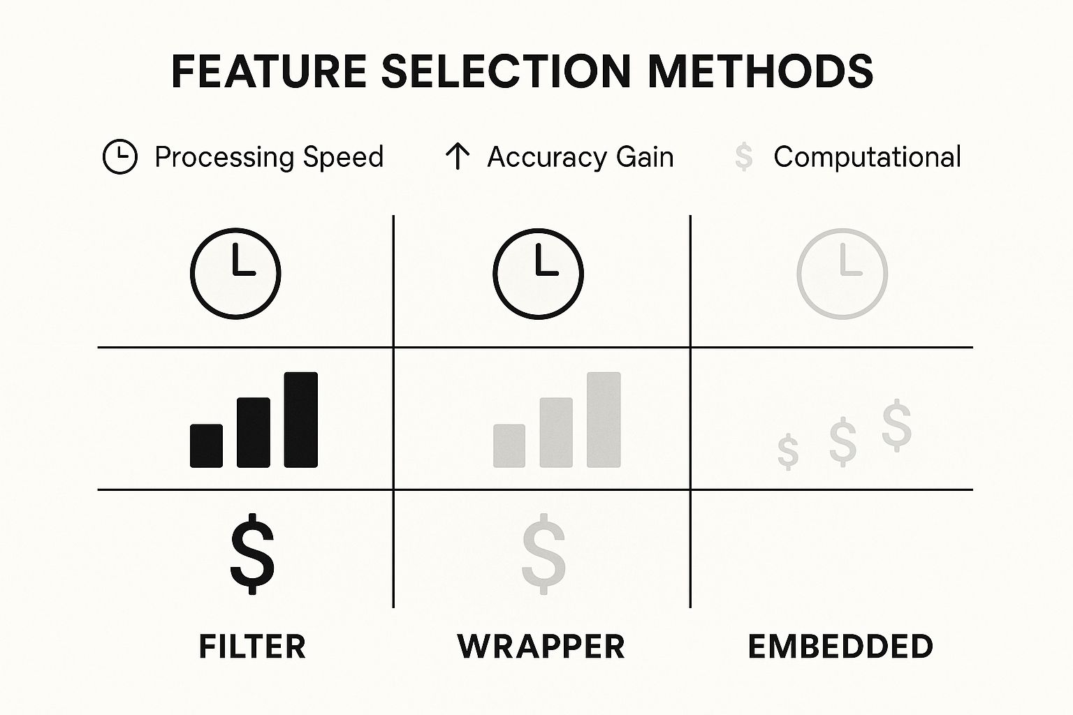
As you can see, Filter methods are lightning-fast but might only give you a modest accuracy boost. Wrapper methods are much slower but can squeeze out the highest performance. Embedded methods offer a great middle ground.

Let’s quickly break down what these methods do:

• Filter Methods: These are the sprinters of feature selection. They are incredibly fast and don't depend on any specific model. They work by using statistical tests (like correlation or Chi-squared) to rank features based on how well they relate to your target variable. You just set a threshold and filter out the weakest ones. Simple and effective.
• Wrapper Methods: Think of these as the marathon runners. They’re much more thorough but also more computationally demanding. Wrapper methods treat feature selection like a search problem, trying out different combinations of features and scoring them based on how well your actual model performs. They "wrap" the selection process around your algorithm to find the optimal feature set.
• Embedded Methods: These are the triathletes, combining training and selection into a single, efficient process. Certain algorithms like LASSO Regression or Random Forests have built-in mechanisms that automatically assign an importance score to each feature as they train. This lets the model itself decide which features are the most impactful.

By mastering both scaling and selection, you ensure your model isn't just powerful but also efficient and reliable. For a deeper dive, check out our guide on feature selection techniques to sharpen your skills even further.

A Practical Feature Engineering Walkthrough

Theory is great, but seeing it all click together in a real project is where the magic happens. Let's get our hands dirty and walk through a feature engineering process from start to finish. We’ll take a raw, messy dataset and transform it into a high-octane, model-ready asset, showing just how much of a difference smart feature engineering techniques can make.

Our mission is to predict housing prices. We'll start with a typical raw dataset and systematically apply the methods we've discussed to clean, enrich, and sharpen it. Each step will come with Python code snippets using pandas and scikit-learn, plus the "why" behind every decision. Think of this as a blueprint you can tear apart and rebuild for your own projects.

Setting the Stage: The Initial Dataset

Let's say our housing dataset has a few core columns: YearBuilt, TotalBsmtSF (total basement square feet), GrLivArea (above-ground living area), and our target, SalePrice. A quick glance shows the usual suspects: missing values, features with wildly different scales, and a ton of untapped potential.

Before we do anything else, we have to split the data. This is non-negotiable. It prevents data leakage, a sneaky problem where information from your test set contaminates the training process, leading to a model that looks great on paper but fails in the real world.

import pandas as pd
from sklearn.model_selection import train_test_split

# Assume 'data' is our initial DataFrame
X = data.drop('SalePrice', axis=1)
y = data['SalePrice']

X_train, X_test, y_train, y_test = train_test_split(X, y, test_size=0.2, random_state=42)

With our data safely partitioned, we can start engineering our features, working only with the X_train set to define our transformations.

Step 1: Creating New Features from Existing Data

Our raw features are a decent starting point, but the real power comes from creating new, more insightful signals.

• House Age: The YearBuilt is okay, but a house's age is a much more direct indicator of its condition and value. So, we'll create a new HouseAge feature.
• Total Square Footage: A buyer doesn't care about basement and above-ground space separately; they care about the total livable area. We'll combine TotalBsmtSF and GrLivArea into a single TotalSF feature.
• Has Remodel: If we have a YearRemodAdd column, we can create a binary feature WasRemodeled that is 1 if YearRemodAdd is different from YearBuilt, and 0 otherwise. This captures a valuable event.

Let's put this into code.

# Create HouseAge feature (assuming current year is 2024)
X_train['HouseAge'] = 2024 - X_train['YearBuilt']
X_test['HouseAge'] = 2024 - X_test['YearBuilt']

# Create TotalSF feature
X_train['TotalSF'] = X_train['TotalBsmtSF'] + X_train['GrLivArea']
X_test['TotalSF'] = X_test['TotalBsmtSF'] + X_test['GrLivArea']

These simple additions inject a ton of context into the data—context a model would really struggle to learn on its own.

Step 2: Handling Missing Values and Scaling

Next up, data quality. Let's imagine our TotalBsmtSF column has some missing values. A solid, straightforward strategy is to fill them with the median value calculated from the training set. We'll also scale our numerical features using StandardScaler to make sure one feature doesn't dominate the model just because its numbers are bigger.

from sklearn.impute import SimpleImputer
from sklearn.preprocessing import StandardScaler

# Impute missing basement square footage
imputer = SimpleImputer(strategy='median')
X_train['TotalBsmtSF'] = imputer.fit_transform(X_train[['TotalBsmtSF']])
X_test['TotalBsmtSF'] = imputer.transform(X_test[['TotalBsmtSF']]) # Use the same imputer

# Scale numerical features
scaler = StandardScaler()
numerical_features = ['HouseAge', 'TotalSF']
X_train[numerical_features] = scaler.fit_transform(X_train[numerical_features])
X_test[numerical_features] = scaler.transform(X_test[numerical_features])

Actionable Insight: Notice we use fit_transform only on the training data. The "rules" we learned—like the median for imputation or the mean/std for scaling—are then applied to the test data using just transform. This is a critical discipline that prevents data leakage.

The Quantifiable Impact of Feature Engineering

This whole process isn't just busywork; it's the engine of modern machine learning. In fact, it’s not uncommon for data scientists to spend 70-80% of their project time on data prep and feature engineering. That effort pays massive dividends, with studies showing that smart feature engineering can boost predictive accuracy by 10-30%. You can find more data on how feature engineering drives model performance.

By creating intuitive features like HouseAge and TotalSF, we've built a dataset that tells a much richer story. A model trained on this engineered data will almost certainly run circles around one trained on the raw, unprocessed version. It's now equipped to make smarter, more nuanced predictions.

Of course, in a real-world project, the job isn't done. The final step is to keep an eye on these features over time to make sure they're still predictive, a process that ties directly into a robust machine learning model monitoring strategy.

Common Questions About Feature Engineering

As you start weaving more sophisticated feature engineering techniques into your projects, a few common questions and roadblocks always seem to pop up. It happens to everyone. Let's tackle some of the most frequent sticking points so you can sidestep common pitfalls and build much more reliable machine learning models.

My goal here is to cut through the complexity and give you direct, experience-based answers that build your confidence.

How Do I Avoid Data Leakage During Feature Engineering?

Data leakage is one of those sneaky, silent model killers. It happens when information from your test set accidentally contaminates your training set. This gives your model an unfair peek at the answers, making it look amazing in development. But the moment you deploy it against truly new data, its performance completely tanks.

There’s a golden rule to prevent this: always, always split your data into training and testing sets before doing any feature engineering.

Every single preprocessing step—from scaling and encoding to imputation—must be "learned" from the training data alone. For example, if you're standardizing features, you calculate the mean and standard deviation only from X_train. Then, you use that same fitted scaler to transform both X_train and X_test. Never, ever fit a preprocessor on the entire dataset.

Is Feature Engineering Still Relevant with Deep Learning?

Yes, absolutely. It's a common misconception that deep learning has made manual feature engineering obsolete.

While it's true that deep learning models are incredible at automatic feature extraction—especially with unstructured data like images or text—they don't make handcrafted features useless. For tabular data, the kind you see every day in business, features built from solid domain knowledge almost always give model performance a significant boost.

Think of it as a partnership, not a competition. Well-crafted manual features provide high-level, context-rich signals that can guide a deep learning model. This makes its job easier and its learning process more efficient. Even with images, you might normalize pixel values. With text, you might create better embeddings. These initial steps give the model a much better starting point. This kind of strategic preparation is a cornerstone of effective data-driven decision making, ensuring your models are built on the strongest possible foundation.

What Is the Difference Between Feature Engineering and Feature Selection?

They sound alike and work together, but they are two very different steps in a machine learning workflow.

• Feature Engineering is the creative process. It’s about creating new features or transforming existing ones to make them more useful. Think combining length and width to get area, or extracting the day_of_week from a date. The goal is to enrich and expand your dataset with more powerful information.

• Feature Selection comes next. It's the analytical process of choosing the best features from the larger pool you now have (including all the new ones you just engineered). The goal here is to cut through the noise, reduce complexity, and prevent overfitting by ditching redundant or irrelevant features.

In short: engineering makes the features, and selection picks the winners. Our blog on feature selection techniques covers this in greater detail.

How Much Feature Engineering Is Too Much?

There's a delicate balance between creating insightful features and just creating noise. The single biggest risk of going overboard with feature engineering is overfitting. If you generate too many highly specific or complex features, your model might start to "memorize" the quirks in your training data instead of learning the real, generalizable patterns. This is often tied to the "curse of dimensionality."

So how do you find that sweet spot? The answer lies in a rock-solid validation strategy.

Actionable Insight: Treat feature creation as an iterative process. Add a new feature, and immediately test its impact on your model's performance using a hold-out validation set. If the feature improves your validation score, great—keep it. If it does nothing or, worse, makes performance drop, get rid of it. Simplicity is your friend. Start with the most intuitive features and build out from there, constantly checking your work against data the model hasn't seen before.

---

At DATA-NIZANT, we are committed to providing expert-led insights that demystify complex data science and AI topics. Explore our in-depth articles to sharpen your skills and drive meaningful results in your projects. Discover more at https://www.datanizant.com.