Unlocking the Power of Feature Selection

In machine learning, choosing the right feature selection techniques is critical for model success. Too many or too few features can negatively impact performance. This listicle presents seven key feature selection techniques to improve your model's accuracy, reduce training time, and enhance interpretability. Learn how to leverage methods like Filter, Wrapper, and Embedded approaches, along with PCA, RFE, LASSO, and Mutual Information, to identify the most impactful features for your data. This knowledge empowers you to build more efficient and effective machine learning models.

1. Filter Methods (Univariate Selection)

Filter methods represent a crucial family of feature selection techniques used in machine learning to enhance model performance, reduce computational complexity, and improve interpretability. These methods are particularly attractive due to their speed and simplicity, making them an excellent starting point in any feature selection workflow. They operate by independently evaluating each feature based on its intrinsic properties and relationship with the target variable, without involving the chosen machine learning algorithm. This independent evaluation is what distinguishes them as 'univariate' selection methods. Essentially, filter methods assign a score to each feature based on a statistical measure – such as correlation, chi-square, information gain, or ANOVA – and then select the top-ranked features based on predefined criteria or thresholds.

How filter methods work is straightforward: calculate a statistical score for each feature reflecting its relevance to the target variable. For example, in a classification problem with categorical features, a chi-square test can measure the dependence between each feature and the target class. In a regression problem, Pearson correlation can quantify the linear relationship between each feature and the continuous target variable. Features are then ranked according to their scores, and the highest-scoring features are selected for model training. This preprocessing step effectively reduces the dimensionality of the dataset before it's fed into a learning algorithm.

Several real-world applications demonstrate the effectiveness of filter methods. For instance, the chi-square test is frequently employed for feature selection in text classification tasks, identifying the most relevant words or n-grams for predicting document categories. Pearson correlation finds application in regression problems, selecting features that show strong linear relationships with the target variable, such as predicting house prices based on features like area and location. In medical diagnostics, ANOVA F-value can be used for feature ranking, identifying biomarkers most significantly associated with a disease. Similarly, Mutual Information is often employed in gene expression analysis, pinpointing genes highly informative about a particular biological process or condition.

Tips for effective implementation:

• Start simple: Use filter methods as an initial step for dimensionality reduction, especially when dealing with high-dimensional datasets.
• Combine metrics: Don't limit yourself to a single metric. Explore different statistical measures and combine their results for a more robust selection.
• Threshold optimization: Determine appropriate threshold values for feature selection based on domain knowledge or cross-validation techniques.
• Statistical assumptions: Be mindful of the specific assumptions of each filter method (e.g., normality for ANOVA) and ensure your data meets those requirements.

Pros:

• Computational efficiency: Filter methods are computationally fast and scale well to high-dimensional data, making them suitable for large datasets.
• Model-agnostic: They are independent of the learning algorithm and can be used with any machine learning model.
• Simplicity: Easy to implement and interpret, requiring minimal parameter tuning.
• Reduced overfitting: Less prone to overfitting compared to more complex feature selection methods like wrapper methods.

Cons:

• Feature independence: Ignores feature dependencies and interactions, potentially missing valuable information.
• Redundancy: May select redundant features, as each feature is evaluated individually.
• Multivariate patterns: Cannot detect complex multivariate patterns that might involve combinations of features.
• Accuracy limitations: Often less accurate than wrapper or embedded methods, particularly when feature interactions are crucial.

Filter methods deserve a prominent place in any feature selection toolkit due to their speed, simplicity, and scalability. While they might not capture the full complexity of feature relationships, they provide a valuable first step in dimensionality reduction, especially when dealing with massive datasets. Their model-agnostic nature also makes them highly versatile, applicable across a wide range of machine learning tasks. Works like Guyon and Elisseeff's "An Introduction to Variable and Feature Selection" and readily available tools like scikit-learn's feature_selection module in Python and R's FSelector package further contribute to their widespread adoption and utility among data scientists and machine learning practitioners.

2. Wrapper Methods

Wrapper methods represent a sophisticated approach to feature selection techniques, distinguished by their use of a machine learning model to evaluate the effectiveness of different feature subsets. Unlike filter methods, which rely on statistical measures, wrapper methods treat the model as a black box, using its predictive performance as the primary criterion for selecting features. They systematically search through the space of possible feature combinations, training and testing the model with each subset to identify the optimal configuration. This process, often guided by search algorithms like forward selection, backward elimination, or recursive feature elimination, allows wrapper methods to implicitly consider feature interactions and dependencies.

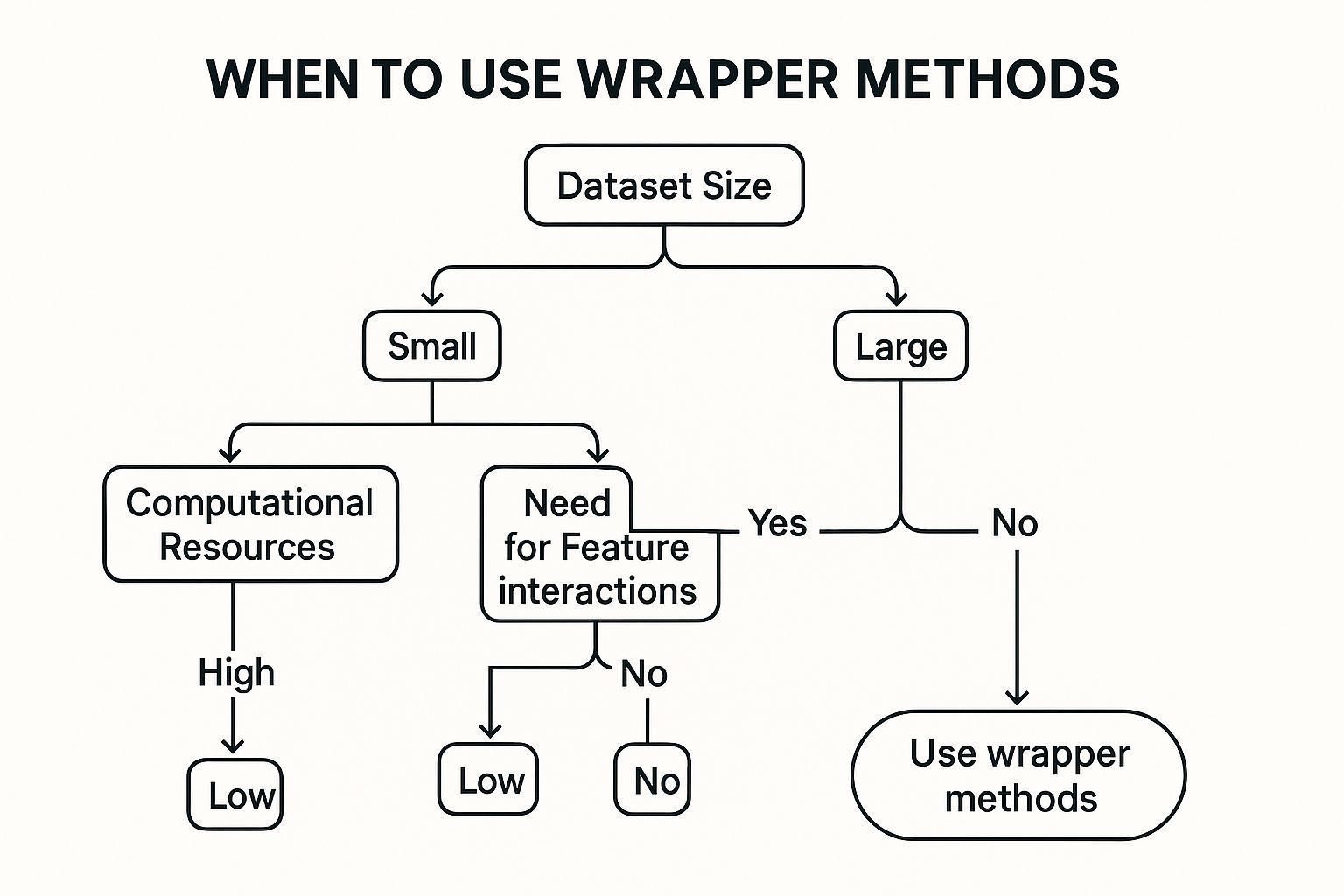
The infographic above visualizes a simplified decision process for employing wrapper methods. It starts with assessing the size of the dataset and the computational resources available. For smaller datasets with ample resources, exhaustive search might be feasible. However, with larger datasets or limited resources, heuristic search methods are preferred. The next decision point involves choosing between forward selection, backward elimination, or recursive feature elimination based on the desired balance between computational cost and accuracy.

Wrapper methods earn their place among feature selection techniques due to their potential for superior predictive performance. By directly optimizing the feature subset for the target model, they can identify compact sets of highly relevant features, leading to improved model accuracy and efficiency. This model-specific optimization makes them particularly useful when feature interactions play a significant role in prediction. Examples of successful implementations include Recursive Feature Elimination (RFE) with Support Vector Machines (SVMs) for gene selection in cancer classification, Sequential Feature Selection in financial market prediction models, and genetic algorithm-based feature selection in fraud detection systems. You can learn more about Wrapper Methods.

Features and Benefits:

• Uses the predictive performance of a model to assess feature subsets: This allows for a more accurate evaluation of feature relevance compared to filter methods.
• Employs search algorithms: Efficiently explores the feature space, identifying optimal subsets even in high-dimensional data.
• Considers feature interactions implicitly: Captures complex relationships between features that might be missed by filter methods.
• Model-specific selection process: Optimizes features specifically for the chosen model, maximizing its performance.

Pros:

• Often yields better predictive performance than filter methods.
• Captures feature interactions and dependencies.
• Optimizes features specifically for the target algorithm.
• Can identify smaller, more effective feature subsets.

Cons:

• Computationally intensive, especially with large feature sets.
• Higher risk of overfitting, particularly with small datasets.
• Results are specific to the chosen model.
• Can be impractical for extremely high-dimensional data.

Tips for Implementing Wrapper Methods:

• Use cross-validation: Mitigates the risk of overfitting, especially with limited data.
• Start with filter methods: Pre-select a smaller subset of features to reduce the computational burden on wrapper methods.
• Consider computational trade-offs when choosing search algorithms: Balance the need for accuracy with the available resources.
• Implement early stopping criteria: Reduces computation time by halting the search when performance improvements plateau.
• Try different search strategies and compare results: Experiment with various algorithms and parameters to find the optimal approach for your specific problem.

The development and popularization of wrapper methods can be attributed to the pioneering work of researchers like Ron Kohavi and George H. John, and John Langley. Tools like the WEKA machine learning toolkit and the mlxtend library by Sebastian Raschka have further facilitated their widespread adoption in the data science community. Wrapper methods offer a powerful approach to feature selection, particularly when predictive accuracy is paramount and computational resources allow for their effective application. They play a vital role in enhancing model performance and driving insights across various domains, from healthcare and finance to fraud detection and natural language processing.

3. Embedded Methods

Embedded methods represent a powerful class of feature selection techniques that seamlessly integrate the selection process into the model training itself. Unlike filter methods, which pre-select features independently of the model, or wrapper methods, which iteratively evaluate feature subsets with the model, embedded methods incorporate feature selection directly into the algorithm's objective function or learning process. This approach cleverly balances the trade-off between model performance and complexity by penalizing models that utilize too many features, effectively combining the advantages of filter and wrapper methods while mitigating their limitations. This makes embedded methods a compelling option for efficient and effective feature selection, particularly with high-dimensional datasets.

Embedded methods achieve this balance primarily through regularization techniques. Regularization adds a penalty term to the model's loss function, discouraging the model from relying too heavily on any single feature and pushing it to select only the most relevant ones. The strength of this penalty, controlled by a hyperparameter, determines the sparsity of the model, i.e., how many features are effectively used. By tuning this hyperparameter, we can control the trade-off between model complexity and performance, effectively performing feature selection during training. This inherent feature selection capability is why embedded methods deserve a prominent place in the suite of available feature selection techniques.

The benefits of embedded methods are numerous. They are generally more computationally efficient than wrapper methods, as they involve only a single model training process. Like wrapper methods, they can capture feature interactions, considering the combined effect of features on the model's performance. Furthermore, the regularization inherent in embedded methods provides a natural defense against overfitting, leading to more robust models. This efficiency and ability to handle interactions make them particularly well-suited for high-dimensional data, where wrapper methods can become computationally prohibitive.

However, embedded methods also have certain limitations. They are often model-specific, meaning the selected features might not be directly transferable to a different algorithm. Implementing embedded methods from scratch can be more complex than filter methods, requiring a deeper understanding of the underlying algorithms and regularization techniques. The interpretation of feature importance can also be more nuanced than with simpler filter methods. While less susceptible than wrapper methods, they can still struggle with extremely high-dimensional data where the sheer number of features presents a significant computational challenge.

Several powerful machine learning algorithms leverage embedded methods for feature selection. LASSO (Least Absolute Shrinkage and Selection Operator) regression, frequently employed in healthcare predictive models, performs feature selection by shrinking the coefficients of less important features to zero. Random Forest, a popular ensemble method used in applications like ecological modeling, provides feature importance scores based on how much each feature contributes to the overall predictive power of the model. Elastic Net, a hybrid approach combining LASSO and Ridge regression, is commonly used in genomic data analysis for its ability to handle correlated features. Gradient boosting algorithms, widely applied in customer churn prediction, also offer embedded feature importance metrics based on feature contributions to the model's boosting stages.

Tips for Effective Use:

• Tune regularization parameters carefully using cross-validation: The regularization parameter significantly influences the feature selection process, and its optimal value should be determined empirically using cross-validation to avoid overfitting or underfitting.
• Compare feature importance across multiple runs for stability: Particularly with algorithms like Random Forests, running the model multiple times and comparing the feature importance rankings can help identify consistently important features and mitigate the effects of randomness.
• Consider the specific biases of each algorithm's importance measure: Different algorithms use different criteria for calculating feature importance. Understanding these biases is crucial for interpreting the results correctly. For example, tree-based methods like Random Forest can be biased towards continuous features or features with many categories.
• Use permutation importance to validate built-in feature importance metrics: Permutation importance provides a model-agnostic way to assess feature importance by measuring the decrease in model performance when a feature's values are randomly shuffled. This helps validate the feature rankings obtained from the algorithm's built-in importance measures.
• Combine with domain knowledge to interpret results: While statistical measures are essential, incorporating domain expertise can enrich the interpretation of selected features and provide valuable insights.

Embedded methods, popularized by researchers like Robert Tibshirani (LASSO), Trevor Hastie and Rob Tibshirani (Elastic Net), and Leo Breiman (Random Forest importance), are readily available in popular machine learning libraries like scikit-learn. Their integrated approach to feature selection offers a powerful and efficient solution for building robust and interpretable models, particularly when dealing with complex datasets in domains such as healthcare, ecology, genomics, and customer relationship management.

4. Principal Component Analysis (PCA)

Principal Component Analysis (PCA) is a powerful dimensionality reduction technique widely employed in feature selection, particularly when dealing with high-dimensional data. It achieves this by transforming the original features into a new set of uncorrelated variables called principal components. These components are essentially linear combinations of the original features, ordered by the amount of variance they explain in the data. While technically a feature extraction rather than a selection method, PCA effectively reduces dimensionality by allowing you to select a subset of the most important components that capture the majority of the variance, thus making it a valuable tool in the feature selection arsenal. This reduction simplifies the data while preserving the most relevant information, leading to improved model performance, faster training times, and reduced computational costs. PCA is particularly relevant in the era of "big data," where datasets often contain hundreds or even thousands of features.

PCA leverages an orthogonal transformation, meaning the principal components are uncorrelated to each other. The first principal component captures the largest amount of variance in the data, the second captures the second largest, and so on. This ordered nature of the principal components allows for a strategic selection process, where components contributing minimally to the overall variance can be discarded without significant information loss. This is a key advantage in feature selection techniques, as it allows for simplification without sacrificing predictive power.

PCA is an unsupervised technique, meaning it doesn't require target variables. This makes it applicable to a wide range of data exploration and preprocessing tasks, including dimensionality reduction for unsupervised learning algorithms like clustering. The ranking of components by explained variance allows data scientists to prioritize features based on their contribution to the overall data structure.

Features of PCA:

• Creates new features (principal components) as linear combinations of original features.
• Orthogonal transformation preserving maximum variance.
• Unsupervised technique, not requiring target variables.
• Components ranked by variance explained.

Pros:

• Removes multicollinearity: Eliminates correlations between features, simplifying the model and improving interpretability (of the components themselves).
• Reduces dimensionality: Preserves the most relevant information while discarding less important features.
• Works well with numerical data: Particularly effective with datasets exhibiting linear relationships between features.
• Efficient for visualization: Reduces high-dimensional data to two or three principal components for easier visualization.

Cons:

• Transformed features lose interpretability: The principal components are linear combinations of original features and may not have direct, real-world meaning.
• Assumes linear relationships between variables: May not be optimal for datasets with complex non-linear relationships.
• Sensitive to feature scaling: Requires standardization or normalization of data before application to ensure that features with larger scales don't dominate the analysis.
• May not preserve class separability in classification tasks: Dimensionality reduction can sometimes lead to a loss of information relevant for class separation.

Examples of Successful Implementation:

• Face recognition (eigenfaces): PCA is used to reduce the dimensionality of face images while preserving essential features for recognition.
• Gene expression data analysis: Identifying key genes and patterns in high-dimensional gene expression data.
• Financial time series dimensionality reduction: Simplifying complex financial data for modeling and forecasting.
• Image compression: Reducing the size of images while preserving essential visual information.

Tips for Effective Use:

• Always standardize/normalize data before applying PCA: This prevents features with larger scales from disproportionately influencing the results.
• Select components based on cumulative variance explained (often 80-95%): This balances dimensionality reduction with information preservation.
• Use scree plots to identify the optimal number of components: Scree plots visualize the explained variance of each component, aiding in selection.
• Consider kernel PCA for non-linear relationships: Kernel PCA extends PCA to handle non-linear data.
• Use incremental PCA for large datasets that don't fit in memory: Incremental PCA processes data in batches, enabling analysis of very large datasets.

PCA's ability to efficiently reduce dimensionality while preserving crucial information makes it a crucial tool in feature selection techniques. Its widespread use across various domains, from computer vision to bioinformatics, highlights its versatility and effectiveness. By following the tips outlined above and understanding its limitations, data scientists and machine learning practitioners can leverage PCA to significantly improve the performance and efficiency of their models.

5. Recursive Feature Elimination (RFE)

Recursive Feature Elimination (RFE) is a powerful feature selection technique that deserves its place among the top methods for optimizing machine learning models. It falls under the category of wrapper methods, meaning it leverages the performance of a machine learning model to assess the importance of features. This approach makes it particularly effective in identifying the optimal feature subset for a specific predictive task and uncovering feature interactions that simpler methods might miss. RFE is especially relevant for data scientists, machine learning engineers, and anyone working with high-dimensional data where identifying key predictors is crucial for model accuracy and interpretability.

How RFE Works:

RFE operates through an iterative backward selection process. It begins by training a model on the complete set of features. Using the model's inherent feature importance ranking (e.g., coefficient magnitudes in linear models, feature importance scores from tree-based models), RFE identifies the least important feature and removes it. This process is repeated recursively, retraining the model and eliminating features one by one until the desired number of features is reached. This iterative elimination allows RFE to capture complex relationships between features, as the importance of each feature is reassessed in the context of the reduced feature set at each step.

Features and Benefits:

• Iterative backward selection approach: Systematically eliminates less important features for improved model performance.
• Model-based feature ranking: Utilizes the model's internal mechanisms to understand feature importance in the context of the prediction task.
• Model agnostic: Can be used with a variety of models that provide feature importance scores, including linear models, support vector machines, and tree-based algorithms.
• Automatic feature subset selection (with cross-validation): The RFECV variant uses cross-validation to determine the optimal number of features, eliminating the need for manual tuning.

Pros:

• Captures feature interactions: By recursively evaluating feature importance, RFE considers how features contribute to model performance in combination with others.
• Optimal subset identification: RFECV automates the process of finding the best number of features.
• Stability: The iterative nature makes RFE more robust to data noise and outliers compared to single-pass feature selection methods.
• Versatility: Works well with both linear and non-linear models.

Cons:

• Computational cost: Can be expensive for datasets with a very large number of features.
• Model dependence: Results are tied to the performance and biases of the chosen base model.
• Sensitivity to noise: While more stable than some methods, RFE can still be affected by noisy data.
• Hyperparameter tuning: Requires careful tuning of the base model's hyperparameters for optimal performance.

Examples of Successful Implementation:

• Gene selection for cancer classification with SVM-RFE: Identifying key genes contributing to cancer development for improved diagnosis and treatment.
• Neuroimaging feature selection for Alzheimer's disease prediction: Selecting relevant brain regions from fMRI or PET scans for early disease detection.
• Sensor selection in IoT applications: Optimizing sensor deployments by identifying the most informative sensors for a specific monitoring task.
• Biomarker identification in medical diagnostics: Discovering key biomarkers for disease diagnosis and prognosis.

Tips for Effective Use:

• Cross-validation with RFECV: Use RFECV to determine the optimal number of features automatically.
• Subset testing: For computationally intensive tasks, start by implementing RFE on a smaller subset of the data.
• Model comparison: Compare RFE results across different base models to assess robustness and gain insights into feature importance from different perspectives.
• Bootstrapping for stability: Evaluate feature stability by running RFE on multiple bootstrapped samples of the data.
• Pre-filtering for high-dimensional data: For extremely high-dimensional data, consider using filter methods (e.g., variance threshold, univariate feature selection) to reduce the initial feature space before applying RFE.

Popularized By:

Isabelle Guyon et al.'s work on "Gene Selection for Cancer Classification using Support Vector Machines" significantly contributed to the popularization of RFE. Efficient implementations of RFE and RFECV are available in scikit-learn (Python) and the Caret package (R). These tools make RFE accessible to a wide range of users and contribute to its continued relevance in the field of feature selection.

6. LASSO (Least Absolute Shrinkage and Selection Operator)

LASSO, short for Least Absolute Shrinkage and Selection Operator, is a powerful feature selection technique that earns its place on this list due to its ability to simultaneously perform variable selection and regularization. This dual functionality leads to improved prediction accuracy and generates more interpretable models, making it a favorite among data scientists and machine learning practitioners. In essence, LASSO helps us identify the most important features in a dataset while preventing overfitting. It achieves this by adding a penalty to the ordinary least squares loss function of a linear regression model. This penalty is proportional to the sum of the absolute values of the model's coefficients, a concept known as L1 regularization.

How does this penalty lead to feature selection? Imagine a model with many features. The L1 penalty encourages the model to minimize the size of the coefficients. Because of the absolute value in the penalty, some coefficients are driven to exactly zero. Features with zero coefficients are effectively removed from the model, thus performing automatic feature selection. The strength of this penalty, and therefore the amount of shrinkage, is controlled by a regularization parameter (often denoted as lambda or alpha).

LASSO is particularly beneficial when dealing with high-dimensional datasets, where the number of features exceeds the number of observations. In such scenarios, traditional regression methods can struggle with overfitting. LASSO's ability to shrink coefficients and eliminate irrelevant features allows it to build more robust models, even when data is sparse. This is crucial for avoiding spurious correlations and ensuring that the model generalizes well to unseen data.

Features and Benefits:

• L1 regularization: This core feature directly leads to the shrinking and zeroing of coefficients, performing the automatic feature selection.
• Combines regression with automatic feature selection: Streamlines the model building process by integrating feature selection directly within the regression.
• Controls model complexity: The regularization parameter allows for fine-tuning the model's complexity, finding a balance between fitting the training data and generalizing to new data.
• Linear model with feature selection capabilities: Extends the capabilities of standard linear models by adding a powerful feature selection mechanism.
• Provides interpretable models with fewer features: Simplifies the model by reducing the number of features, making it easier to understand and explain.

Pros and Cons:

Pros:

• Automatically performs feature selection during model training.
• Helps prevent overfitting by constraining model complexity.
• Effective for high-dimensional, sparse datasets.
• Provides interpretable models with fewer features.

Cons:

• May struggle with highly correlated features (tends to pick one).
• Requires careful tuning of the regularization parameter.
• Limited to linear relationships between features and target.
• Can be sensitive to feature scaling.

Examples of Successful Implementation:

• Gene expression analysis for disease prediction: Identifying key genes related to specific diseases from thousands of potential candidates.
• Financial predictive modeling with many potential indicators: Selecting the most influential economic factors for predicting market movements.
• Text classification with large feature spaces: Reducing the dimensionality of text data by selecting the most relevant words or n-grams.
• Neuroimaging studies for identifying relevant brain regions: Pinpointing the brain areas most associated with certain cognitive functions.

Actionable Tips:

• Always normalize features before applying LASSO: This ensures that features are on a similar scale and prevents the penalty from being unfairly applied.
• Use cross-validation to tune the regularization parameter: This helps find the optimal balance between model complexity and prediction accuracy.
• Consider Elastic Net for highly correlated features: Elastic Net combines L1 and L2 regularization and can handle correlated features more effectively.
• Examine stability of selected features across multiple runs: This helps assess the robustness of the feature selection process.
• Implement feature standardization to ensure fair penalty application: Consistent scaling across features is important for the L1 penalty to work as intended.

Learn more about LASSO (Least Absolute Shrinkage and Selection Operator)

LASSO has been popularized by Robert Tibshirani (introduced in 1996), with significant contributions from Trevor Hastie and Rob Tibshirani through their influential textbooks. Practical implementations are readily available through the glmnet package in R and the linear_model module within scikit-learn in Python. Its widespread use across various domains underscores its effectiveness as a crucial technique for feature selection.

7. Mutual Information

Mutual Information (MI) earns its place among the top feature selection techniques due to its powerful ability to identify non-linear relationships between features and the target variable. This filter-based method, rooted in information theory, quantifies the statistical dependency between two variables. Essentially, it measures how much knowing the value of one variable reduces uncertainty about the other. This makes it a versatile tool for identifying relevant features for both classification and regression tasks, regardless of whether the relationships are linear.

How Mutual Information Works

Unlike correlation, which primarily detects linear relationships, MI can capture complex dependencies. It achieves this by calculating the shared information content between two variables. A high MI score indicates a strong relationship, suggesting the feature is highly informative about the target variable. This information-theoretic approach is particularly valuable when dealing with real-world datasets, where relationships are often more nuanced than simple linear correlations.

Advantages and Disadvantages of Mutual Information

MI boasts several advantages as a feature selection technique:

• Captures Non-linear Dependencies: A key strength of MI is its ability to identify non-linear relationships that linear methods like correlation would miss. This makes it applicable to a broader range of datasets and problems.
• Model-Agnostic: As a filter method, MI operates independently of any specific machine learning algorithm. It acts as a preprocessing step, selecting features that can then be used with any model. This enhances flexibility and simplifies the workflow.
• Computational Efficiency: Compared to computationally intensive wrapper methods, MI is relatively fast to compute, making it suitable for larger datasets.
• Versatile Applicability: MI works effectively with both numerical and categorical features, broadening its applicability across various data types.

However, MI also has some limitations:

• Multivariate Interactions: MI primarily focuses on pairwise relationships and doesn't inherently account for complex interactions between multiple features.
• Discretization Challenges: While MI can handle both continuous and discrete variables, applying it to continuous data often requires discretization, which can introduce sensitivity to binning strategies and estimator parameters.
• Small Sample Size Issues: In high-dimensional datasets with limited samples, MI can become unreliable and susceptible to overfitting.
• Estimator Sensitivity: The choice of estimator for continuous data can impact the results, requiring careful consideration and potentially experimentation.

Examples of Successful Implementation

Mutual Information has proven effective in various domains:

• Text Feature Selection: In natural language processing, MI helps identify keywords and phrases most relevant to a specific topic or sentiment.
• Genomic Data Analysis: MI can be used to discover biomarkers and identify genes associated with specific diseases.
• Image Feature Selection: In computer vision, MI helps select image features that are most discriminative for object recognition or image classification tasks.
• Sensor Data Selection: In Internet of Things (IoT) applications, MI can identify the most informative sensor readings for predictive maintenance or anomaly detection.

Tips for Effective Use

To maximize the benefits of MI, consider the following tips:

• Estimator Selection: Experiment with different estimators for continuous data, such as kernel density estimation or k-nearest neighbors, particularly for smaller datasets.
• Handling Feature Interactions: Combine MI with other techniques, like feature importance from tree-based models, to capture multivariate interactions.
• Normalization: Normalize MI scores to a range between 0 and 1 for better interpretability and comparison across features.
• Visualization: Visualize feature relationships to validate the results and gain a deeper understanding of the selected features. Learn more about Mutual Information (While this link points to an article on LIME, it could be helpful in the context of interpretability, especially when combined with feature selection.)
• Combined Approach: Consider using MI alongside other feature selection techniques to get a more robust set of features.

When to Use Mutual Information

Mutual Information is a valuable tool when:

• Non-linear relationships are suspected: If you believe linear correlations might not capture the full complexity of the relationships in your data.
• A model-agnostic approach is desired: When you want to select features independently of the chosen machine learning algorithm.
• Computational efficiency is important: For larger datasets where wrapper methods might be too computationally expensive.
• Dealing with both numerical and categorical data: When your dataset contains a mix of data types.

By understanding the strengths and limitations of Mutual Information and employing the tips provided, data scientists and machine learning practitioners can effectively leverage this powerful technique to improve model performance and gain valuable insights from their data.

Feature Selection Methods Comparison

Technique	Implementation Complexity 🔄	Resource Requirements ⚡	Expected Outcomes 📊	Ideal Use Cases 💡	Key Advantages ⭐
Filter Methods (Univariate Selection)	Low – statistical scoring only	Low – computationally efficient	Fast dimensionality reduction, quick filtering	Initial feature reduction, high-dimensional data	Model-agnostic, simple, scalable
Wrapper Methods	High – involves model training & search	High – compute-intensive	High predictive accuracy, considers feature interactions	Small to medium datasets, when feature interactions matter	Optimizes for specific model, captures dependencies
Embedded Methods	Medium – integrated in model training	Medium – single model training	Balanced accuracy and feature reduction	When using specific algorithms with built-in selection	Efficient, less prone to overfitting
Principal Component Analysis (PCA)	Medium – matrix operations, eigen decomposition	Medium – depends on data size	Reduced dimensionality with uncorrelated components	Linear, numerical data, visualization, data compression	Removes multicollinearity, preserves variance
Recursive Feature Elimination (RFE)	High – iterative training and elimination	High – several training cycles	Optimal feature subset, model-specific	When using models with feature importance, moderate dataset size	Captures interactions, stable subset selection
LASSO (Least Absolute Shrinkage and Selection Operator)	Medium – regularized linear model	Medium – single model training	Sparse, interpretable models	High-dimensional regression, sparse datasets	Automatic selection, reduces overfitting
Mutual Information	Low – information-theoretic measures	Low – efficient calculation	Detects non-linear dependencies	Preprocessing for varied data types, non-linear relations	Captures complex relationships, model-agnostic

Choosing the Right Feature Selection Approach

Effectively utilizing feature selection techniques is crucial for building robust and efficient machine learning models. From filter methods like univariate selection and mutual information, to wrapper methods, embedded methods like LASSO and RFE, and dimensionality reduction techniques like PCA, the variety of approaches covered in this article provides a powerful toolkit for any data scientist. Remember that each technique has its strengths and weaknesses. Filter methods are computationally efficient but may overlook complex feature interactions. Wrapper methods offer higher accuracy but can be computationally expensive. Embedded methods cleverly integrate feature selection within the model training process, while PCA helps reduce dimensionality and noise.

Mastering these feature selection techniques is essential for several reasons. By reducing the number of irrelevant or redundant features, we enhance model interpretability, decrease training time, mitigate overfitting, and ultimately improve model performance. Measuring the effectiveness of your feature selection method is crucial. Consider tracking key metrics such as accuracy, precision, recall, and F1-score. For a deeper dive into performance measurement, check out this helpful resource on content performance metrics.

The best approach depends heavily on your specific dataset, computational resources, and project goals. Selecting the right technique often involves experimentation and careful evaluation. Unlock the full potential of your data and streamline your machine learning workflows. Visit DATA-NIZANT to discover how our platform simplifies and automates feature selection, empowering you to build high-performing models with efficiency and ease.