
If you've spent any time in data science, you know the old saying: "garbage in, garbage out." It's a cliché for a reason. Messy, inconsistent data can silently sabotage everything you build, from simple marketing dashboards to sophisticated machine learning models. It leads to bad insights, flawed decisions, and wasted resources.
This is where data cleaning in Python becomes your most valuable—and frankly, most underrated—skill. It's the unglamorous but absolutely essential process of finding and fixing the errors, inconsistencies, and inaccuracies in a dataset. Using powerful libraries like Pandas and NumPy, you transform raw, chaotic information into a reliable asset. This isn't just a preliminary step; it's where projects are won or lost.
Why Data Cleaning Is Your Most Valuable Skill

Think of this guide as your practical playbook. We're moving beyond the theory to give you actionable workflows for data cleaning in Python that you can apply immediately. We’ll be focusing on the core data science libraries that professionals use every day to get the job done.
The Growing Need for Clean Data
The sheer amount of data being created is hard to wrap your head around. By 2025, the world is expected to generate around 175 zettabytes of it. This explosion of information makes automated and accurate data cleaning more critical than ever. With over 40% of data science tasks now being automated, the quality of the data fed into those systems is the single biggest factor for success.
The consequences of ignoring data quality are serious. In fact, studies show that roughly 60% of organizations grapple with ethical dilemmas from AI-driven decisions that can be traced directly back to poor data. This highlights just how central data cleaning is to mitigating both reputational and financial risk.
Actionable Insight: Data cleaning isn't just about fixing errors; it's about building trust in your data. As you'll see in our guide on data cleaning best practices, every inconsistent entry you correct and every missing value you address strengthens the integrity of your entire analysis.
What to Expect From This Guide
My goal here is to show you how mastering data cleaning directly makes you a more effective and valuable data professional. We'll walk through the entire process using real-world scenarios, complete with Python code and clear explanations for tackling common data quality headaches.
We're going to cover a complete workflow, from start to finish:
- Initial Data Inspection: Learning how to get a quick feel for a new dataset and spot problems at a glance.
- Handling Missing Values: Exploring different strategies—and when to use each—for dealing with gaps in your data.
- Correcting Inconsistencies: Standardizing formats, fixing typos, and resolving other structural errors.
- Managing Outliers: Deciding what to do with those strange data points that just don't seem to fit.
This guide provides a comprehensive, hands-on learning path. For a deeper dive into some of the foundational concepts, you can also check out this detailed guide on data cleaning in Python, which is a great companion to the practical steps we'll cover here.
Your First Look at a Messy Dataset

Before you can fix anything, you need to play detective. The very first step in any real-world data cleaning python workflow isn't about writing code to fix problems—it's about finding them. You have to get a feel for the data's structure, understand the kinds of errors you're dealing with, and pinpoint where the biggest messes are. This initial exploratory phase guides every single decision you'll make later on.
Let's dive right in with a practical example. Say we have a customer_data.csv file. It's full of the usual suspects: missing details, columns with the wrong data types, and inconsistent text. Our first job is to load it into a Pandas DataFrame, which is the absolute workhorse for data manipulation in Python.
import pandas as pd
import numpy as np

# Practical Example: Create a messy DataFrame to simulate real-world data
data = {
    'customer_id': [101, 102, 103, 104, 105, 106, 107, 101],
    'signup_date': ['2022-01-15', '2022-01-16', None, '2022-01-18', '2022-01-19', '2022-01-20', '2022-01-21', '2022-01-15'],
    'total_spend': ['$55.00', '60', '75.50', '$80.00', '90', '15000', '-50', '$55.00'],
    'customer_age': [25, 30, 22, 150, 45, 33, np.nan, 25],
    'country': ['USA', 'U.S.A.', 'Canada', 'USA', 'United States', 'Canada', 'Mexico', 'USA']
}
df = pd.DataFrame(data)
With the data loaded, our investigation can officially begin.
Running an Initial Health Check
The first command I run, almost reflexively, is .head(). It’s simple, but it gives you an immediate glimpse of the first five rows. You get a quick sense of the columns and the data they hold, letting you visually scan the landscape.
# Practical Example: Display the first 5 rows of the DataFrame
print("Initial Data Preview:")
print(df.head())
This one command can often reveal obvious problems right off the bat. You might spot a customer_id that should be a number but has weird characters, or a signup_date that’s clearly not a standard date format.
For a deeper, more technical summary, the next tool is .info(). This method is incredibly powerful for diagnosing issues hiding just beneath the surface. It provides a concise summary, showing each column's data type and, crucially, how many non-null values it contains.
# Practical Example: Get a summary of the DataFrame
print("\nDataFrame Info:")
df.info()
The output from .info() is where the real detective work heats up. If you see a column with 8 entries but only 6 non-null values for customer_age, you’ve just uncovered 2 missing records that need attention. Likewise, if total_spend shows up as an object (text) instead of a float64 (a number), you know there are non-numeric characters like dollar signs lurking in there, ready to break any calculations.
Actionable Insight: The output of
.info()essentially becomes your data cleaning to-do list. Every mismatched data type and column with missing values is a task you need to check off. As we discuss in our post on data-driven decision making, this initial checklist is your first step toward building a reliable dataset.
Getting a Statistical Overview
While .info() tells us about the structure, .describe() gives us a statistical summary of the numerical columns. It instantly calculates the count, mean, standard deviation, min, max, and quartile values.
# Practical Example: Generate descriptive statistics for numerical columns
print("\nStatistical Summary:")
print(df.describe())
This output is a goldmine for spotting anomalies and getting a sense of your data's distribution. Here’s what I look for:
- Check the
count: Does it match across all columns? If not, it confirms the missing values you likely already spotted with.info(). - Compare
meanandmedian(the 50% mark): If the mean is way higher than the median, it's a big clue that your data is skewed right, probably because of some high-value outliers. - Look at
minandmax: Do these numbers even make sense in the real world? Acustomer_agewith amaxof 150 is obviously an error. Apurchase_amountwith aminof -50 also points to a serious data entry problem.
This initial diagnostic phase—combining .head(), .info(), and .describe()—doesn't fix a single thing. And that's the point. It’s all about building a comprehensive picture of the problems you're up against. You’ve now identified the exact issues—missing values, incorrect data types, and potential outliers—that we’ll start tackling in the next sections.
Handling Missing Data with Pandas
After that first health check of your data, you’re almost guaranteed to find missing values. These gaps aren't just minor annoyances; they're a real threat to the quality of your analysis. Knowing how to deal with them is a cornerstone of any good data cleaning python workflow, and this is where the Pandas library really comes into its own.
The first move is always to get a clear picture of the problem. A simple .isnull().sum() gives you a direct count of missing values per column.
# Practical Example: Count missing values in each column
print("Missing values per column:")
print(df.isnull().sum())
This simple command immediately tells you that signup_date is missing one value and customer_age is missing another. Seeing this pattern is key to making a smart decision about what to do next.
To Drop or to Fill: The Core Dilemma
When you find missing data, you're faced with two main choices: get rid of it (deletion) or fill it in (imputation). There's no single "best" answer. The right call depends entirely on your specific dataset and goals. The aim is to minimize any damage to your data's integrity while making it usable for your models.
A good way to frame your thinking is to look at the percentage of missing data and what kind of data it is.
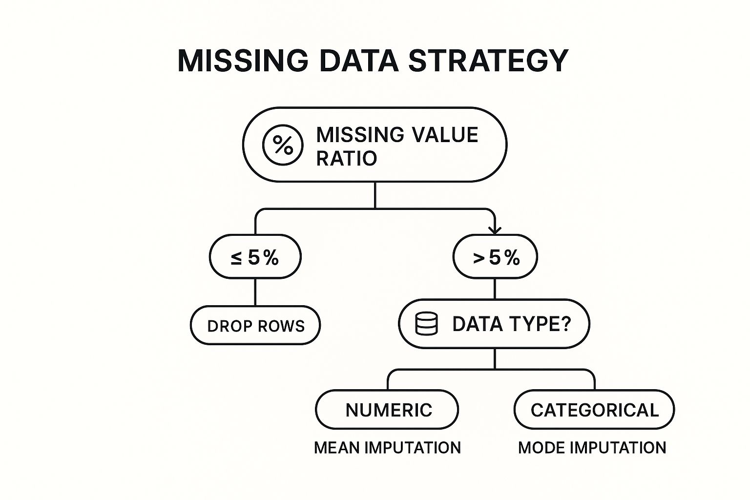
This decision tree gives you a solid rule of thumb. If you've got just a small amount of missing data, dropping those rows is usually fine. But for bigger gaps, you need a more thoughtful approach like imputation.
Deletion with dropna()
If a column is missing just a few values—say, less than 5%—and you have a large dataset, dropping the affected rows is often the easiest and safest route. It's clean, quick, and probably won't introduce any serious bias.
# Practical Example: Drop any row that has a missing value in 'signup_date'
# This is often critical, as a signup date might be essential for analysis.
df_dropped = df.dropna(subset=['signup_date'])
print("\nDataFrame after dropping rows with missing signup_date:")
print(df_dropped)
But be careful here. If a single column is missing 30% of its values, a blanket dropna() will wipe out a massive chunk of your data, taking perfectly good information from other columns along with it.
The Art of Imputation with fillna()
When dropping data isn't an option, you turn to imputation—the technique of filling in the blanks. The Pandas fillna() method is incredibly powerful and gives you several smart ways to do this.
Choosing Your Missing Data Strategy
Deciding how to fill missing values is a critical step. The right method depends on your data's characteristics and what you're trying to achieve. Here’s a quick comparison of the most common strategies in Pandas to help you choose.
| Method | Pandas Function | Best Use Case | Potential Drawback |
|---|---|---|---|
| Drop Rows/Columns | .dropna() |
Small % of missing data; non-critical features. | Can cause significant data loss if overused. |
| Fill with Mean | .fillna(df['col'].mean()) |
Numerical data with a normal distribution. | Sensitive to outliers, which can skew the result. |
| Fill with Median | .fillna(df['col'].median()) |
Skewed numerical data or data with outliers. | May not represent the "true" center for all distributions. |
| Fill with Mode | .fillna(df['col'].mode()[0]) |
Categorical data. | Can introduce bias if one category is too dominant. |
| Forward Fill | .fillna(method='ffill') |
Time-series data where values are assumed to be constant. | Can propagate an incorrect value over a long gap. |
| Backward Fill | .fillna(method='bfill') |
Time-series data where future values are known. | Not suitable for real-time data where future is unknown. |
Each method has its place. The key is to think critically about the nature of your data and the potential impact of your choice before applying a fix.
Using Statistical Measures
For numerical columns, the go-to strategies are filling with the mean, median, or mode.
- Mean: Works well for normally distributed data without big outliers.
- Median: A much better choice for skewed data, as it isn't thrown off by extreme values.
- Mode: Can be used for numbers, but it's really the top choice for categorical columns.
# Practical Example: Fill missing 'customer_age' values with the median
median_age = df['customer_age'].median()
df['customer_age'].fillna(median_age, inplace=True)
print(f"\nMissing 'customer_age' values filled with median: {median_age}")
print(df)
Actionable Insight: Choosing between the mean and median isn't just a technicality; it's a decision that shapes the story your data tells. For a column like
income, using the mean could artificially inflate the average, whereas the median gives a much more realistic picture of a "typical" value.
Advanced Filling Techniques
For some data, simple stats just don't cut it. Think about time-series data, like daily sales. If Wednesday's number is missing, filling it with the overall average is probably wrong. In cases like this, forward-fill or backward-fill make a lot more sense.
- Forward-fill (
ffill): Fills a missing value with the last known one. Perfect for when you can assume a value holds steady until the next measurement. - Backward-fill (
bfill): Fills a missing value with the next known one.
# Practical Example: Create a time-series column and use ffill
df_ffill = pd.DataFrame({'date': pd.to_datetime(['2023-01-01', '2023-01-02', '2023-01-03', '2023-01-04']),
                         'stock_price': [150, np.nan, 152, np.nan]})
df_ffill['stock_price_ffill'] = df_ffill['stock_price'].fillna(method='ffill')
print("\nForward-fill example:")
print(df_ffill)
The power and flexibility of Python for these kinds of tasks are a huge reason for its dominance in data science. In fact, 53% of developers now use Python for data science, largely because libraries like Pandas are so good at tackling missing data—a problem that crops up in up to 20% of real-world datasets. Getting good with functions like fillna() and dropna() can cut your data processing time by up to 40% compared to manual methods, which directly boosts the quality of your final analysis.
Ultimately, handling missing data is a blend of technical skill and good judgment. Mastering these techniques is fundamental to building a clean, reliable dataset that supports sound data-driven decision making.
Fixing Inconsistent and Inaccurate Data

Okay, let's move beyond just filling in missing values. The next, and arguably more subtle, layer of data cleaning is all about fixing the errors that are actually in your dataset. I’m talking about the sneaky issues: duplicate records, text entries that mean the same thing but are spelled differently, and data types that just don't make sense. These are the kinds of problems that can silently sabotage your analysis. It's not just a minor annoyance, either—poor data quality can cost organizations an average of $12.9 million a year from bad decisions based on flawed insights. This is where we shift from filling gaps to actively correcting the data we have.
Eliminating Structural Errors with drop_duplicates()
Duplicate rows are one of the most common Gremlins you'll find in raw data. They can artificially inflate your numbers, mess up your averages, and make it look like you have more customers or transactions than you really do. In our example DataFrame, customer_id 101 appears twice.
Luckily, Pandas gives us a straightforward way to hunt down and eliminate these redundant entries.
# Practical Example: Check for duplicate rows
duplicate_rows = df.duplicated()
print(f"Number of duplicate rows: {duplicate_rows.sum()}")

# Remove duplicate rows based on all columns
df.drop_duplicates(inplace=True)
print("\nDataFrame after removing duplicates:")
print(df)
Using inplace=True is memory-efficient because it modifies the DataFrame directly. A word of caution, though: it's often safer to create a copy and work on that until you're confident your cleaning logic is solid.
Actionable Insight: Get familiar with the
subsetparameter indrop_duplicates(). Sometimes, a row is only a true duplicate if certain key columns match, likecustomer_idandsignup_date. This gives you fine-grained control over what you define as a duplicate in your specific context.
Standardizing Inconsistent Text Data
Inconsistent text is another classic data cleaning headache. Our country column has entries like 'USA', 'U.S.A.', and 'United States'. To your Python script, these are three completely different categories, which will wreak havoc on any grouping or filtering.
This is a perfect job for Python's string methods and the .replace() function in Pandas.
# Practical Example: Create a mapping for inconsistent country names
print("\nUnique country values before standardization:")
print(df['country'].unique())

country_mapping = {
    'U.S.A.': 'USA',
    'United States': 'USA'
}

# Apply the mapping to the 'country' column
df['country'] = df['country'].replace(country_mapping)
print("\nUnique country values after standardization:")
print(df['country'].unique())
This approach is easy to read and super effective for inconsistencies you already know about. For more widespread issues like random capitalization or extra whitespace, you can chain string methods together for a quick fix.
Correcting Mismatched Data Types
Ever tried to calculate the average of a column of numbers, only to get an error? It’s probably because they're stored as text (an object dtype in Pandas), like our total_spend column with its dollar signs. This is a total roadblock for any math.
The .astype() method is your go-to tool here.
# Practical Example: Remove dollar signs and convert 'total_spend' to a numeric type
print("\n'total_spend' dtype before conversion:", df['total_spend'].dtype)
df['total_spend'] = df['total_spend'].replace({'\$': ''}, regex=True).astype(float)
print("'total_spend' dtype after conversion:", df['total_spend'].dtype)
print(df.head())
For dates, Pandas has the incredibly smart pd.to_datetime() function. It's surprisingly good at parsing various date formats without you having to specify them.
# Practical Example: Convert 'signup_date' column from string to datetime objects
df['signup_date'] = pd.to_datetime(df['signup_date'], errors='coerce')
print("\n'signup_date' dtype after conversion:", df['signup_date'].dtype)
I almost always use errors='coerce'. It’s a safe way to handle any dates that just can't be parsed; it turns them into NaT (Not a Time), which you can then treat just like any other missing value. These small, targeted fixes are fundamental to solid data cleaning best practices.
Preparing Data for Machine Learning with Scaling
Once the data is clean, you might need to take one final step, especially if you're building a machine learning model. Many algorithms can get thrown off if your features are on wildly different scales. Think about customer_age (from 22-45) and total_spend (from 55-15000 in our messy data). The spend values would completely dominate.
Data scaling brings all your features to a similar scale. Scikit-learn has two fantastic tools for this:
StandardScaler: This rescales your data to have a mean of 0 and a standard deviation of 1.MinMaxScaler: This rescales data into a specific range, usually 0 to 1.
# Practical Example: Use MinMaxScaler on numerical features
from sklearn.preprocessing import MinMaxScaler

# First, handle the obvious outliers for a more meaningful scaling
df = df[df['total_spend'] < 1000] # Remove the extreme outlier

scaler = MinMaxScaler()
numerical_features = ['customer_age', 'total_spend']

df[numerical_features] = scaler.fit_transform(df[numerical_features])
print("\nDataFrame after scaling numerical features:")
print(df)
This final transformation is about more than just cleaning—it's about optimizing your data for advanced analysis. It's the step that ensures your models are built on a fair, reliable, and solid foundation.
Identifying and Managing Outliers
Outliers are the silent saboteurs of data analysis. These extreme data points can drastically skew statistical measures, mislead visualizations, and ultimately corrupt your machine learning models. In our data, customer_age of 150 and total_spend of 15000 and -50 are clear outliers. Any robust data cleaning python strategy has to include a clear plan for finding and dealing with them.
The real challenge with outliers is that they aren't always errors. Sometimes they represent a rare but totally valid event. Your job isn't just to blindly delete them. It’s to investigate, understand the context, and choose a path that fits your analytical goals.
Visual Detection with Plots
Before you write a single line of statistical code, trust your eyes. Data visualization is an incredibly powerful way to make outliers literally pop off the screen.
- Box Plots: These are the gold standard for spotting outliers. Any points that fall way outside the plot's "whiskers" are immediately flagged.
- Scatter Plots: When you're looking at the relationship between two numerical variables, a scatter plot is your best friend.
import seaborn as sns
import matplotlib.pyplot as plt

# Practical Example: A box plot to find outliers in 'customer_age'
# We'll use the original messy data to see the outliers clearly
original_df = pd.DataFrame(data)
original_df['total_spend'] = original_df['total_spend'].replace({'\$': ''}, regex=True).astype(float)
original_df['customer_age'].fillna(original_df['customer_age'].median(), inplace=True)


print("\nVisualizing Outliers:")
plt.figure(figsize=(12, 5))
plt.subplot(1, 2, 1)
sns.boxplot(x=original_df['customer_age'])
plt.title('Box Plot of Customer Age')

plt.subplot(1, 2, 2)
sns.boxplot(x=original_df['total_spend'])
plt.title('Box Plot of Total Spend')
plt.show()
These simple plots give you an intuitive feel for your data's distribution and help you confirm if outliers are a real problem you need to solve programmatically.
A Statistical Approach with IQR
Visual inspection is great, but for a systematic way to flag outliers, we can lean on the Interquartile Range (IQR). This is a classic and reliable technique for defining outlier boundaries based on the data's own spread.
The process is quite straightforward:
- Calculate the first quartile (Q1) and third quartile (Q3).
- Calculate the IQR (
IQR = Q3 - Q1). - Define your upper and lower bounds, typically 1.5 * IQR below Q1 and above Q3.
Any data point falling outside these computed bounds is tagged as an outlier.
# Practical Example: Identify outliers in 'customer_age' using IQR
Q1 = original_df['customer_age'].quantile(0.25)
Q3 = original_df['customer_age'].quantile(0.75)
IQR = Q3 - Q1
lower_bound = Q1 - 1.5 * IQR
upper_bound = Q3 + 1.5 * IQR

outliers = original_df[(original_df['customer_age'] < lower_bound) | (original_df['customer_age'] > upper_bound)]
print("\nOutliers detected using IQR method:")
print(outliers)
Actionable Insight: The decision of what to do with an outlier is more art than science. It requires a blend of statistical evidence, domain knowledge, and a clear understanding of your project's objectives, a key theme in our machine learning in marketing guide. Removing a data point that represents a legitimate, albeit rare, customer could be a huge mistake.
Strategic Outlier Management
Okay, so you’ve identified your outliers. What’s next? You have a few options, and the right choice is always highly contextual.
-
Removal: If you're confident an outlier is just a data entry error (like an age of 150 or spend of -50), getting rid of it is often the cleanest solution.
-
Capping (Winsorization): This is a less extreme option. It involves capping the outlier values at a certain percentile. For instance, you could replace all values above the 99th percentile with the value at the 99th percentile.
-
Transformation: For skewed data, applying a mathematical transformation like a log function can pull in high-value outliers and make the distribution more normal.
# Practical Example: Removing clear errors
cleaned_df = original_df[(original_df['customer_age'] < 100) & (original_df['total_spend'] > 0)]

print("\nDataFrame after removing outliers (age > 100, spend < 0):")
print(cleaned_df)
Ultimately, managing outliers is a critical thinking exercise. The methods you use in your data cleaning python script should be defensible and well-documented. Your goal is to ensure the final dataset is both clean and truly representative of the phenomenon you're studying.
Common Questions About Data Cleaning in Python
As you get your hands dirty with more projects, you'll inevitably hit some roadblocks and start questioning the best way to handle certain data cleaning python tasks. These aren't just textbook problems; they're the practical hurdles every single data pro has to clear. Getting solid, actionable answers is how you build both confidence and speed.
Let's walk through some of the most common questions that pop up when you're in the trenches cleaning data.
What Is the Difference Between Data Cleaning and Data Transformation?
I like to think of it like renovating a house.
Data cleaning is the essential repair work. You're patching holes in the walls (handling missing values), tossing out junk left by the previous owners (removing duplicates), and fixing foundational issues (correcting data entry errors). The goal is to make sure the structure is sound, stable, and accurately represented.
Data transformation, on the other hand, is the remodeling you do for a specific purpose. This might mean knocking down a wall to create an open-concept living space (engineering new features from existing ones) or upgrading the wiring to handle modern appliances (scaling numbers with normalization or standardization).
You almost always clean the data before you transform it. Cleaning ensures accuracy; transformation preps the data for a specific model or analysis.
Should I Drop a Row with Missing Data or Fill It?
The honest answer? It depends entirely on the context and the potential impact.
If you have a massive dataset and only a tiny fraction of rows—say, under 5%—have missing values, dropping them is often a quick, low-risk move. It’s unlikely to introduce any serious bias into your analysis.
But, if dropping those rows would mean losing a significant chunk of your data or skewing its overall distribution, imputation (filling in the missing values) becomes the smarter play. Your choice of what to fill it with is just as critical.
- For skewed numerical data, use the median. It’s much less sensitive to outliers than the mean.
- For categorical data, the mode (the most frequent value) is your best bet.
Choosing correctly is a balancing act. You have to weigh the need for data integrity against maintaining a large enough sample size for your models to learn from.
Can I Fully Automate My Python Data Cleaning Pipeline?
While it’s tempting to write a script that does everything with one click, a completely "hands-off" automated pipeline is rarely a good idea. So many data cleaning decisions demand human judgment and a bit of domain expertise.
For instance, an automated script might spot a huge sales figure, flag it as an outlier, and delete it. But what if that wasn't an error? It could have been a legitimate, game-changing transaction. This is where a human-in-the-loop approach shines.
Go ahead and automate the predictable, repetitive stuff:
- Trimming whitespace from text columns.
- Converting known date formats.
- Applying standard fixes for inconsistent categories (like mapping "USA" and "U.S.A." to a single value).
But always, always build in checkpoints for manual review, especially when dealing with outliers or complex inconsistencies. This balanced approach is a cornerstone of effective data science project management, ensuring that your quest for efficiency doesn't sacrifice accuracy.
Actionable Insight: The goal of a good data cleaning script isn't to replace the analyst, but to empower them. It should handle the tedious work, freeing you up to focus on the nuanced decisions that require human intelligence.
Which Library Is Better for Data Cleaning: Pandas or NumPy?
For the hands-on work of a data cleaning python workflow, Pandas is your go-to tool, period. It was built from the ground up to handle tabular data using its incredibly intuitive DataFrame object. High-level functions like fillna(), dropna(), and drop_duplicates() make the most common cleaning tasks straightforward and easy to read.
So where does NumPy fit in? It's the high-performance engine that Pandas is built on top of. NumPy is a beast when it comes to fast, efficient numerical computations on arrays, and it forms the foundation of Python's entire scientific computing ecosystem.
While NumPy is what makes Pandas so fast, you'll be interacting directly with Pandas for almost every cleaning task—from reading data to finding and fixing issues. Think of it this way: Pandas is the car you drive, and NumPy is the powerful engine under the hood.
At DATA-NIZANT, we believe that mastering the foundational skills of data science is key to unlocking powerful insights. Our expert-authored articles and guides break down complex topics into actionable knowledge, helping you navigate everything from data preparation to advanced AI. Explore more at https://www.datanizant.com to sharpen your skills.

