
If you're looking to break into data science, the single most impactful skill you can learn first is SQL (Structured Query Language). It's the universal key that unlocks the vast majority of valuable company data, letting you directly query, filter, and shape information to generate actionable insights long before you even think about firing up Python or R for analysis.
Why SQL Is Your Most Valuable Skill in Data Science

Before you write a single line of Python, it’s worth understanding why SQL is the absolute bedrock of a data scientist's toolkit. This isn't some dusty, legacy tool; it's the active, living language for talking to relational databases, which is where most businesses keep their most important assets.
This direct access is what really matters. The reality of any data science project is that an enormous chunk of your time goes into just getting and preparing the data. Being good at SQL directly speeds up this process, which is often the biggest bottleneck you'll face.
The Language of Business Data
Just think about where a company's most prized information lives:
- Customer purchase histories
- Website user activity logs
- Product inventory levels
- Financial transaction records
All this critical data is almost always sitting in structured databases. SQL is the bridge that connects your analytical goals to this raw information. Without it, you’re stuck waiting for data engineers to hand you flat files like CSVs—a process that can be slow, inefficient, and leave you with stale data.
To give you a quick reference, here's a table summarizing the core SQL concepts we'll be diving into and why they're indispensable for any data scientist.
Core SQL Concepts for Data Scientists at a Glance
| SQL Concept | Primary Use Case in Data Science | Actionable Insight |
|---|---|---|
SELECT and WHERE |
Filtering and extracting specific subsets of data. | Reduces data volume before analysis, making Python/R processing much faster. |
JOIN |
Combining data from multiple tables (e.g., users and orders). | Creates a complete, unified view needed for comprehensive analysis. |
GROUP BY and Aggregates |
Summarizing data (e.g., calculating averages, sums, counts). | The foundation of most business intelligence and reporting tasks. |
| Window Functions | Performing calculations across a set of table rows. | Essential for complex analyses like cohort analysis or calculating running totals. |
| Subqueries/CTEs | Breaking down complex queries into logical, readable steps. | Helps manage complexity and makes code maintainable and easier to debug. |
This table is just a high-level map. The real power comes from seeing these concepts in action, which is exactly what we’ll cover.
Actionable Insight: SQL remains a foundational skill because it is the native language of the systems holding the most valuable data. Being fluent means you can explore, understand, and shape datasets at their source, giving you more control and speed.
Efficiency and Scalability
Top companies list SQL as a non-negotiable skill for one simple reason: efficiency. Running your filters, joins, and aggregations directly in the database is drastically faster than pulling a massive, multi-gigabyte table into a pandas DataFrame and then trying to wrestle with it.
Practical Example: You need to find the total sales for a specific product category ('Electronics') from last month. With SQL, you write a simple query that tells the database to do the heavy lifting:
SELECT SUM(sale_amount)
FROM sales
WHERE category = 'Electronics'
  AND sale_date >= '2024-09-01' AND sale_date < '2024-10-01';
In return, you get a single number—a tiny amount of data. The alternative? Fetching the entire sales table, potentially millions of rows, and then doing the math on your local machine. It’s a night-and-day difference in performance.
This efficiency is also key to preparing clean datasets for machine learning. By using SQL for the initial heavy lifting and data shaping, the work you do later becomes much simpler. As discussed in our guide on data cleaning with Python, a well-structured input from SQL makes subsequent Python steps far more effective. Ultimately, SQL isn't about choosing one tool over another; it’s about building a solid foundation that makes every other part of your job easier.
Setting Up a Realistic Practice Environment

Theory is one thing, but to really master SQL for a data scientist role, you have to get your hands dirty. Abstract concepts only get you so far; the real learning happens when you're working with real tools and messy data to solve tangible problems. Your first and most critical step on this journey is setting up a solid local environment.
The good news? You don't need a pricey enterprise license to get started. Free, industry-standard tools like PostgreSQL and SQLite give you more than enough power to build job-ready skills. My advice is to start with one of these two.
Choosing Your Database
- SQLite is a fantastic starting point. It’s serverless and completely self-contained, storing the entire database in a single file on your machine. This makes the setup incredibly simple, letting you focus on core SQL syntax without getting bogged down in server management.
- PostgreSQL, on the other hand, is a more powerful, open-source object-relational database. It runs on a client-server model, which is a much closer match to what you'll encounter in a real-world enterprise environment. If your goal is to practice with a setup that mirrors a future job, PostgreSQL is the better long-term choice.
Once you have your database management system (DBMS) installed, you'll need some data. Please, skip the classic "employees" and "departments" toy examples. Instead, grab a rich, public dataset from a source like Kaggle—an e-commerce transaction log or a user behavior dataset is perfect. This gives you realistic columns, data types, and challenges to work with.
This choice often mirrors what you'll find at a company. For example, while SQL Server 2019 still commands a 44% market share as of early 2025, the 2022 version has already captured 21% as companies upgrade. Understanding these trends helps you pick tools that are not just powerful but also relevant.
From Installation to Your First Query
With a dataset in hand, the next step is loading it. Most database tools provide a GUI (like DBeaver or pgAdmin) that lets you import a CSV file directly. This process automatically creates a table structure for you, bridging the gap between a flat file and a fully queryable database.
Now for the fun part. Let's run a practical query. Forget "hello world"—we're going to ask a real business question. Assuming we have an e-commerce dataset loaded into a table named transactions, we can find all the unique users who made a purchase in the last 30 days.
Practical Example: Find all unique users who made a purchase on or after September 1st, 2024.
SELECT
  DISTINCT user_id
FROM
  transactions
WHERE
  purchase_date >= '2024-09-01';
This simple query does far more than just pull data; it filters through potentially millions of rows to isolate a specific, relevant subset. The WHERE clause is your primary tool for this, allowing you to ask incredibly precise questions. Learning how to apply these filters at the database level is a core skill we explore further in our guide to applying data science for business.
Actionable Insight: A good practice environment isn’t about complexity; it’s about realism. Using a real-world dataset on a standard database system forces you to solve the same kinds of problems you'll face in your first data science role.
This kind of hands-on experience builds confidence almost immediately. You shift from being a passive learner to an active practitioner, directly translating business questions into functional SQL code and seeing the results for yourself.
Turning Raw Data into Insights with Joins and Aggregations
So far, we've been pulling data from single tables. That's a good start, but the real magic of SQL for a data scientist happens when you start weaving together information from multiple tables. This is how you go from just fetching data to actually generating insights right at the source.
The most crucial tool for this is the JOIN clause. It’s how you connect the dots between related pieces of information that live in different places. For example, you might have a users table with registration dates and a separate login_activity table that tracks every single login. On their own, neither table tells the full story.
Connecting the Dots with JOINs
To get a complete picture of user engagement, you have to combine them. A hands-on example makes this crystal clear. Let's say we want to see the last login date for every user who signed up in the last year. We can pull this off with a simple INNER JOIN.
This flow shows how SQL takes raw, separate data points and transforms them into a cohesive, grouped result—the core of analytical work.
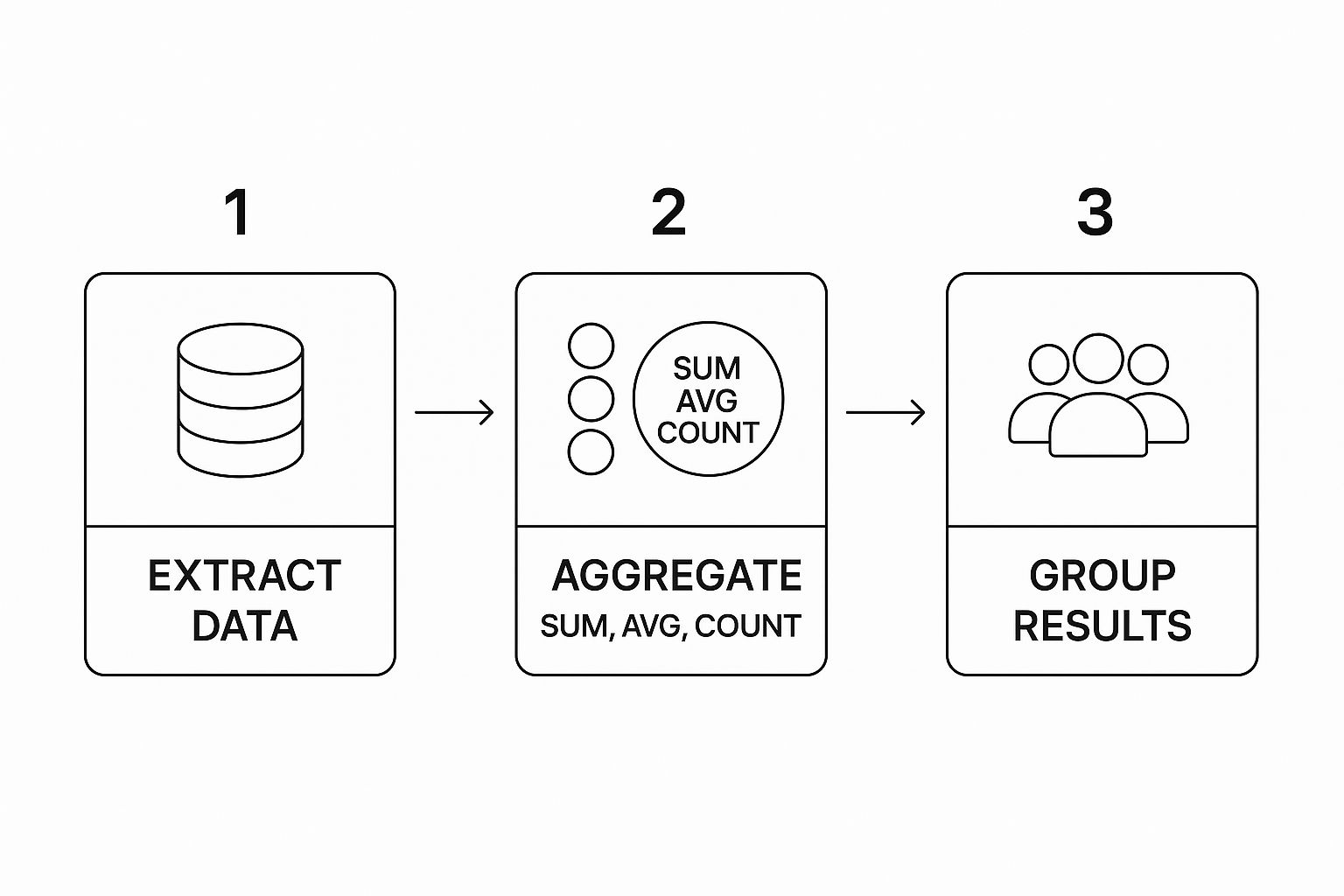
As the visual shows, we first extract the data, apply aggregate functions to summarize it, and then group the results to produce a meaningful final table.
Practical Example: Combine user registration data with their login activity.
-- Combine user registration data with their login activity
SELECT
    u.user_id,
    u.registration_date,
    l.login_timestamp
FROM
    users u
INNER JOIN
    login_activity l ON u.user_id = l.user_id
WHERE
    u.registration_date >= '2023-10-01';
This query links our two tables on the common user_id column, giving us a unified view. But this is just the raw, combined data—it's often way too granular for any real analysis. The next logical step is to summarize it.
Summarizing Data with Aggregations
This is where GROUP BY and aggregate functions like COUNT(), SUM(), and AVG() come into play. These are your workhorses for performing calculations on groups of rows, turning thousands of individual records into a clean, concise summary.
Building on our last query, let's tackle a more practical business question: "For each user, what is their total number of logins and their most recent login date?"
Practical Example: Calculate total logins and find the last login for each user.
-- Calculate total logins and find the last login for each user
SELECT
    u.user_id,
    COUNT(l.login_id) AS total_logins,
    MAX(l.login_timestamp) AS last_login_date
FROM
    users u
INNER JOIN
    login_activity l ON u.user_id = l.user_id
GROUP BY
    u.user_id
ORDER BY
    total_logins DESC;
Look at what we just accomplished. Instead of dragging every single login event into a Python script to do the math, we’ve pushed the heavy lifting to the database. The result is a small, clean, and highly relevant summary table.
Actionable Insight: Performing aggregations directly in SQL is far more efficient than pulling raw data. You reduce network traffic, minimize memory usage in your analytical tool, and get answers much faster. This is a foundational practice when you're working with large datasets.
Metrics like these are incredibly valuable. They can be plugged directly into a dashboard or become the foundation for more advanced analysis. In fact, these aggregated results are often the perfect starting point when you need to master feature engineering techniques for machine learning models. By getting comfortable with JOIN and GROUP BY, you gain the power to ask—and answer—sophisticated questions right inside the database.
Unlocking Deeper Analysis with Window Functions

If GROUP BY is the trusty workhorse of SQL analytics, then window functions are the high-performance engine that separates the pros from the true experts. For any serious sql for data scientist workflow, they're an absolute game-changer, letting you perform complex calculations across a set of related rows while keeping each individual row intact.
That’s a critical distinction. A GROUP BY clause squashes your data down into a single summary row. Window functions, on the other hand, calculate a value—like a rank or a running total—for each row based on its "window," or a group of related rows. This lets you ask much more sophisticated questions without getting tangled up in messy self-joins.
Beyond Basic Aggregations
Let's say you're working with a sales table and need to find the top 5 best-selling products within each product category. With GROUP BY, you could get the total sales per category, but you'd lose all the detail about the individual products.
This is where a function like RANK() comes to the rescue. It lets you partition your data by one column (like category) and then order it by another (like total_sales) to assign a rank to each product inside its group.
Practical Example: Find the top-selling products within each category.
WITH ProductSales AS (
  SELECT
    product_id,
    category,
    SUM(sale_amount) as total_sales
  FROM
    sales
  GROUP BY
    product_id, category
)
SELECT
  product_id,
  category,
  total_sales,
  RANK() OVER (PARTITION BY category ORDER BY total_sales DESC) as sales_rank
FROM
  ProductSales;
That OVER (PARTITION BY category ...) clause is where the magic happens. It tells the RANK() function to start over for each new category, giving you an independent ranking within each one. The final result would show every product, its total sales, and its specific rank within its own category.
Analyzing Sequences and Time Series
Another incredibly powerful use for window functions is analyzing sequential data, a bread-and-butter task for data scientists. Functions like LEAD() and LAG() were practically built for this.
LAG(): Gives you access to data from a previous row in your result set.LEAD(): Lets you peek ahead and access data from a subsequent row.
Think about calculating month-over-month sales growth. Without window functions, this is a surprisingly clumsy task. But with LAG(), it becomes almost trivial. You can pull the previous month's sales figure onto the current month's row and do the math right there.
Practical Example: Compute daily sales variance.
SELECT
  sale_date,
  daily_total,
  LAG(daily_total, 1) OVER (ORDER BY sale_date) as previous_day_total,
  daily_total - LAG(daily_total, 1) OVER (ORDER BY sale_date) as day_over_day_change
FROM
  daily_sales_summary;
This simple, elegant query compares each day's sales to the previous day's in a single pass. The output from this kind of analysis is perfect for spotting trends or anomalies, which is a core part of effective machine learning model monitoring.
Actionable Insight: Use
LEAD()andLAG()to sidestep complicated self-joins when comparing sequential records. This is your go-to method for calculating period-over-period growth, deltas between events, or the time elapsed between user actions.
Getting comfortable with these functions will dramatically expand the kinds of questions you can answer directly in your database. You’ll write cleaner, more efficient queries and showcase a level of SQL skill that will make you stand out in any data science interview.
Integrating SQL into Your Python Workflow
In my experience, a data scientist who stays locked in a single environment just isn't working at full potential. The real magic happens when you fluidly combine the power of SQL with a programming language like Python. Knowing how to bridge this gap isn't just a "nice-to-have"—it's a core skill that separates the efficient data scientists from the rest.
The trick is knowing when to use each tool. The best practice I've always followed is simple: let SQL do the heavy lifting. This means running your large-scale filtering, joining, and aggregations directly on the database server, where it's fastest. Once the data is trimmed down and shaped, you pull that much smaller, pre-processed result into Python for the fun stuff like modeling and visualization.
Connecting Python to Your Database
So, how do you get Python to talk to your database? This is where a couple of essential libraries, SQLAlchemy and pandas, become your best friends. SQLAlchemy is a fantastic toolkit for connecting to just about any SQL database you can think of, while pandas can execute a SQL query and load the results directly into its famous DataFrame structure.
Practical Example: Pull aggregated customer data directly into a pandas DataFrame using a Jupyter Notebook.
import pandas as pd
from sqlalchemy import create_engine

# First, create a database connection engine.
# This example uses SQLite, but you can easily adapt the string for PostgreSQL, MySQL, etc.
db_connection_str = 'sqlite:///your_database_file.db'
db_engine = create_engine(db_connection_str)

# Write your SQL query as a multi-line string.
query = """
SELECT
    customer_id,
    COUNT(order_id) as total_orders,
    SUM(order_value) as total_spend
FROM
    orders
WHERE
    order_date >= '2024-01-01'
GROUP BY
    customer_id
ORDER BY
    total_spend DESC;
"""

# Use pandas to execute the query and load the results right into a DataFrame.
customer_summary_df = pd.read_sql(query, db_engine)

# And just like that, you have a clean, aggregated DataFrame ready for analysis in Python.
print(customer_summary_df.head())
This approach really does give you the best of both worlds. The demanding work is handled by the database server, and Python receives a perfectly structured DataFrame, primed for statistical modeling, machine learning, or creating insightful visualizations.
A Skill with Real-World Demand
Getting comfortable with this integrated workflow isn't just about making your own life easier; it's a direct response to what the market is screaming for. The demand for data scientists who are fluent in both Python and SQL is exploding. In fact, data science roles are expected to see a 28% annual job growth rate by 2025, which could mean around 11.5 million new jobs popping up worldwide. As we've covered before on Datanizant in our post on the future of data science, this specific combination of skills is pure gold.
Actionable Insight: The most effective data scientists don't see SQL and Python as separate tools. They see them as two halves of a single, powerful data pipeline. Let the database handle the scale, and let Python handle the complexity.
This mindset isn't just theory—it reflects the day-to-day reality of a working data professional. By pushing the heavy data crunching to SQL, you drastically cut down on data transfer times and memory usage in your Python environment. It’s simply the smarter, more scalable way to handle production-level data.
Common Questions About SQL for Data Science
As you get deeper into the world of data, you’ll inevitably run into some common questions about where SQL fits in. I’ve heard these from countless aspiring data scientists, so let’s clear them up with some straightforward, practical answers.
Is SQL Still Relevant with NoSQL and Big Data?
Absolutely. It's a question that comes up all the time, especially with the rise of NoSQL databases. While those systems are fantastic for unstructured data like text or images, the fact is that most core business data—customer records, financial transactions, product inventory—still lives in relational databases. SQL is the language for that world.
Actionable Insight: Data scientists spend a massive chunk of their time on data prep. It's far more efficient to use SQL to filter and aggregate huge datasets right at the source, rather than pulling terabytes of raw data into your local machine's memory. It’s never been about "SQL vs. NoSQL"; it's about using the right tool for the job. And for structured data, SQL's role is as critical as ever.
What Is the Difference Between SQL and a Dialect Like T-SQL?
Think of it like this: SQL is the universal language standard, like the blueprint for a car engine. Dialects like Microsoft's T-SQL or Oracle's PL/SQL are specific implementations of that blueprint, built by different manufacturers. They might add a turbocharger or a unique fuel injection system.
All dialects use the core commands you know—SELECT, WHERE, JOIN. But they also add proprietary functions and procedural logic. My advice? Master standard SQL first; it’s a universally transferable skill. But if your company uses a specific dialect, getting familiar with its unique features can give you a real edge by letting you write more powerful, optimized queries.
Should I Aggregate Data in SQL or with Pandas?
The golden rule is to do the heavy lifting in the database whenever you can. For filtering, joining, and aggregating massive tables, SQL will almost always be faster and more resource-efficient. Databases are purpose-built for these kinds of set-based operations.
Actionable Insight: Use SQL to create your clean, aggregated analytical base table. Then, load that much smaller table into pandas for tasks SQL isn't built for, like statistical modeling and achieving machine learning mastery.
Following this approach dramatically reduces the data you have to pull over the network and load into your Python environment, which makes your entire workflow faster and more scalable.
How Much SQL Do I Really Need to Know?
You need to know enough to be self-sufficient. I’ve seen many junior data scientists get stuck because they constantly have to ask a data engineer to pull data for them. Don't be that person.
Actionable Insight: Being self-sufficient means you are comfortable writing queries that:
- Join multiple tables to create a single, unified dataset.
- Perform complex filtering using subqueries or Common Table Expressions (CTEs).
- Use aggregate functions with
GROUP BYto summarize information effectively. - Understand and apply window functions for more advanced analysis, like creating rankings or running totals.
You don’t need to be a database administrator, but you absolutely must be able to independently explore, extract, and shape the data you need. As highlighted in our Datanizant article on applying data science for business, this skill alone makes you incredibly valuable and efficient.
At DATA-NIZANT, we provide expert-authored articles and analysis to help professionals master key skills in data science, AI, and machine learning. Explore our in-depth guides to stay ahead in your field. Visit us at https://www.datanizant.com.

