Ever wonder how a computer learns to "see"? It's not magic, it's a Convolutional Neural Network (CNN). These are a special type of deep learning model built specifically for handling pixel data, which is why they're the absolute standard for things like image classification and object detection.

Instead of just looking at a flat list of numbers, a CNN learns to recognize features in an image, building up its understanding from simple edges all the way to complex objects. This guide will provide actionable insights and practical examples to get you started.

How a CNN Actually Learns to See

Before we jump into any code, it’s really important to get a gut feeling for what a CNN is doing under the hood. Unlike a standard neural network that flattens an image into a long vector of pixels, a CNN is designed from the ground up to respect the spatial structure of an image. It doesn't see a "cat" right away. First, it sees the basic building blocks—edges, textures, shapes, and patterns—that, when pieced together, form the concept of a cat.

This whole idea is inspired by how our own visual cortex works. While the concepts have been around since the 1980s, it was Yann LeCun's LeNet-5 architecture back in 1998 that really put them on the map by successfully reading handwritten digits. Back then, the lack of massive datasets and serious computing power held things back, but the core ideas were solid.

The Building Blocks of a CNN

A CNN is essentially a stack of specialized layers, and each layer has a very specific job to do. If you're just getting started, you might want to check out our guide on neural network basics to get your bearings first. Once you understand what each layer does, building and troubleshooting your own models becomes much more intuitive.

Here are the three main players you'll be working with:

• Convolutional Layers: These are the heart and soul of the network. They use filters (also called kernels) that slide across the input image to hunt for specific features. Early on, these filters might pick up on simple things like vertical lines or color gradients. As you go deeper into the network, the layers learn to combine these simple features into more complex patterns, like an eye or a car's wheel.
• Pooling Layers: Right after a convolutional layer has done its job extracting features, a pooling layer comes in to clean things up. It shrinks the spatial size of the data, usually through a process called max pooling. This makes the network more efficient and helps it focus only on the most significant features that were detected.
• Fully Connected Layers: These sit at the very end of the network. They take all the high-level features extracted by the previous layers and do the final classification. Think of them as the decision-makers that look at the evidence and make the final call, like labeling an image as a "dog" or a "cat."

To make this clearer, here's a quick breakdown of what each layer is responsible for.

Key CNN Layers and Their Functions

Layer Type	Primary Function	Key Analogy
Convolutional	Feature Detection	A detective using different magnifying glasses (filters) to find specific clues (features) like fingerprints or footprints in an image.
Pooling	Downsampling & Dimensionality Reduction	Summarizing a long book into a one-page synopsis. It keeps the most important information while making it much smaller and easier to handle.
Fully Connected	Classification & Decision-Making	The final jury that takes all the evidence presented by the detectives and decides on a verdict ("cat" or "dog").

By stacking these layers, a CNN creates a powerful feature hierarchy. It starts with the tiny details and gradually builds up a more abstract, complete understanding of what's in the image.

The real power of a CNN is that it learns what features to look for on its own. We don't have to manually program it to find edges or textures; it figures out the best filters during the training process.

This automated feature learning is precisely what makes CNNs so incredibly effective for image-related tasks. In the rest of this tutorial, we'll get our hands dirty and actually build each of these layers from scratch.

Getting Your Python Environment Ready for Deep Learning

Before we can even think about building a convolutional neural network, we need to get our workshop in order. A clean, well-organized Python environment is your best friend here—it prevents a world of hurt down the line, letting you focus on the model instead of fighting with package versions. Think of this setup as the launchpad for everything else we'll do in this guide.

The two main tools in our belt will be TensorFlow and Keras. TensorFlow is the heavy-lifter, the powerful backend that handles all the intense number-crunching. Keras, on the other hand, is the friendly API that sits on top, making it much simpler to actually design and build our models. It’s like having a powerful engine with an intuitive dashboard.

Installing the Core Libraries

Getting these libraries installed is pretty straightforward with pip, Python's package manager. I can't stress this enough: for any new project, always start by creating a dedicated virtual environment. It walls off your project's dependencies from your main Python installation, which is a lifesaver for avoiding conflicts.

Once you've created and activated your virtual environment, pop open your terminal and run these two commands:

Install TensorFlow (which now includes Keras)

pip install tensorflow

Install Jupyter for an interactive workspace

pip install notebook

That's it. This simple setup gives you everything you need to start building and experimenting. I'm a big fan of using a Jupyter Notebook for this kind of work. It lets you run small bits of code, see the output immediately, and tweak things on the fly, which is perfect for the iterative nature of deep learning.

As you start writing code, it's a great time to build good habits. A big part of that is managing source code effectively to keep your work organized and track every change you make.

Making Sure Everything Works

With the tools installed, we need to do a quick systems check. The most important test is to see if TensorFlow can find a GPU (Graphics Processing Unit) on your machine. Why does this matter? Training a CNN on a GPU can be anywhere from 10 to 50 times faster than on a CPU. That's the difference between waiting minutes versus hours.

Fire up a Jupyter Notebook and run this little Python script in a cell:

import tensorflow as tf

print("TensorFlow Version:", tf.version)
gpu_devices = tf.config.list_physical_devices('GPU')
if gpu_devices:
print(f"GPU is available: {gpu_devices}")
else:
print("GPU not available, TensorFlow will use CPU.")

If the output says a GPU is available, you're all set for some seriously fast training. If not, no big deal—you can still follow along and complete this entire tutorial using your CPU. It'll just take a bit longer.

A stable environment is non-negotiable for any serious deep learning project. Taking 20 minutes to set this up correctly now will save you hours of debugging later.

Now that our environment is good to go, it's time to get our data in order. Just like any other machine learning project, how you handle your data is absolutely critical. If you want a refresher, our guide on the fundamentals of data preprocessing in machine learning is a great place to start before we jump into building our first model.

Building a CNN for Image Classification From Scratch

Alright, we've covered the theory and have our environment ready to go. Now it's time to roll up our sleeves and actually build something. This is where we bridge the gap between abstract concepts and real, working code. We're going to build a functional image classifier from the ground up using Keras, a wonderfully intuitive API that lives inside TensorFlow. You'll be surprised how straightforward it is to construct a fairly complex network.

Our model's first challenge will be the CIFAR-10 dataset, a classic benchmark in the computer vision world. It’s a collection of 60,000 tiny 32×32 color images spread across ten distinct classes—think 'airplane', 'automobile', 'bird', and 'cat'. Our mission, should we choose to accept it, is to train a CNN that can correctly identify what's in a new image from this dataset.

Loading and Preparing the Data

Before our network can learn anything, we need to get the data into a shape it can understand. This means tackling two essential preprocessing steps: normalization and encoding.

Raw images are just grids of pixel values, typically ranging from 0 to 255. We'll normalize these values by dividing each one by 255, which scales them neatly into a 0 to 1 range. This simple step is a big deal for training stability, as it prevents the optimizer from getting thrown off by wildly different input values.

The image labels ('cat', 'dog', etc.) also need a numerical makeover. We'll use a technique called one-hot encoding. Instead of labeling the 'cat' class as 3, we transform it into a vector where every element is zero except for a 1 at the third position (e.g., [0, 0, 0, 1, 0, 0, 0, 0, 0, 0]). This stops the model from accidentally learning a false order, like assuming a 'dog' is somehow "greater than" a 'cat'.

Let's see what this looks like in Python.

import tensorflow as tf
from tensorflow.keras.datasets import cifar10
from tensorflow.keras.utils import to_categorical

Load the CIFAR-10 dataset

(x_train, y_train), (x_test, y_test) = cifar10.load_data()

Normalize pixel values to be between 0 and 1

x_train = x_train.astype('float32') / 255.0
x_test = x_test.astype('float32') / 255.0

One-hot encode the labels

num_classes = 10
y_train = to_categorical(y_train, num_classes)
y_test = to_categorical(y_test, num_classes)

Designing the CNN Architecture

Now for the fun part: actually designing the model layer by layer. A standard CNN for image classification begins with a series of convolutional and pooling layers to find patterns, then flattens that information to feed into dense layers that make the final call.

This infographic gives a great visual overview of how an image gets processed through convolution and pooling, which are the foundational blocks of our network.

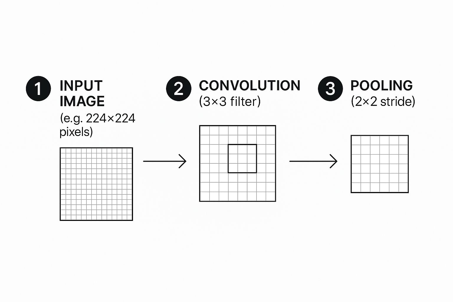
This cycle of feature extraction and downsampling is what allows the network to build a hierarchy of features, starting with simple lines and colors and building up to more complex shapes and objects.

Our model will follow this proven blueprint. We'll stack a few Conv2D layers, each followed by a MaxPooling2D layer. The early convolutional layers will be on the lookout for basic features like edges and gradients. As data flows deeper, later layers will combine these simple patterns to recognize more intricate things like textures or parts of an object.

The number of filters in a convolutional layer is a key hyperparameter to tweak. A common and effective strategy is to start with a smaller number, like 32, and increase it in deeper layers. This lets the network learn a wider variety of more abstract features as it goes.

After the feature extraction stage, a Flatten layer converts the 2D feature maps into a long, 1D vector. This vector is then passed to one or more Dense (or fully connected) layers, which handle the final classification logic.

The very last layer is a Dense layer with a neuron count equal to our number of classes—10 in this case—and a softmax activation function. Softmax is perfect for this job because it converts the network's raw output scores into a set of probabilities that sum to one, giving us a clear prediction for each class. Getting a handle on how different activation functions work is really important; our guide on neural network activation functions dives much deeper into this topic.

The Complete Code for Building the Model

Here’s the full Keras code that defines our CNN architecture. I've added comments to each line to explain not just what it does, but why it's there.

from tensorflow.keras.models import Sequential
from tensorflow.keras.layers import Conv2D, MaxPooling2D, Flatten, Dense

Define the model architecture

model = Sequential()

First Convolutional Block

32 filters of size 3×3, ReLU activation. 'padding="same"' ensures output size is same as input.

'input_shape' is only needed for the first layer.

model.add(Conv2D(32, (3, 3), padding='same', activation='relu', input_shape=(32, 32, 3)))
model.add(MaxPooling2D(pool_size=(2, 2))) # Downsamples the feature map

Second Convolutional Block

We increase the number of filters to 64 to learn more complex features.

model.add(Conv2D(64, (3, 3), padding='same', activation='relu'))
model.add(MaxPooling2D(pool_size=(2, 2)))

Third Convolutional Block

Further increasing filters to 128 for even more abstract feature detection.

model.add(Conv2D(128, (3, 3), padding='same', activation='relu'))
model.add(MaxPooling2D(pool_size=(2, 2)))

Flattening and Classification Layers

model.add(Flatten()) # Converts 3D feature maps to a 1D vector
model.add(Dense(512, activation='relu')) # A dense layer for classification
model.add(Dense(num_classes, activation='softmax')) # Output layer with softmax for probabilities

Print a summary of the model

model.summary()

Running model.summary() is a fantastic habit to get into. It gives you a clean, tabular breakdown of your architecture, showing the output shape and parameter count for every single layer. It's incredibly handy for a quick sanity check or for debugging when things don't look quite right. With our model defined, the next move is to compile and train it, which we'll jump into next.

Getting Your CNN Ready to Train and Evaluate

So far, all we have is a blueprint. Our CNN architecture is defined, but it's an empty shell with no real knowledge. The next step is where the magic happens: we're going to breathe life into it through training.

This is the part where we teach the network how to tell images apart by showing it thousands of examples. We'll start by setting up its learning strategy and then kick off the process of feeding it data.

Compiling Your Model for Learning

Before we can throw data at our model, we need to configure its learning process. In Keras, this is handled by the .compile() method. Think of this as giving our model three things: a teacher, a grading system, and a goal.

Here’s what we need to specify:

• Optimizer: This is the engine that drives the learning, adjusting the model's internal weights to chip away at the error. The Adam optimizer is a fantastic workhorse—it's efficient, easy to configure, and performs well on a huge range of problems.
• Loss Function: This is how we measure how wrong the model is. For a multi-class problem like CIFAR-10 (which has 10 classes), 'categorical_crossentropy' is the perfect fit. It quantifies the gap between the model's predicted probabilities and the actual, one-hot encoded labels.
• Metrics: While the loss function steers the training, metrics are for us humans. They help us track how the model is actually doing in terms we can understand. We’ll monitor 'accuracy' to see the raw percentage of images it gets right.

Putting it all together in code is surprisingly simple.

Compile the model

model.compile(optimizer='adam',
loss='categorical_crossentropy',
metrics=['accuracy'])

That one line of code gets our CNN prepped for the most intensive part of its journey.

Kicking Off the Training Process

With the setup complete, we can finally start the main event using the .fit() method. This is where the model iteratively learns from our training data. We'll hand it our training images (x_train) and their labels (y_train), but we also need to decide on a couple of crucial hyperparameters.

These two settings, epochs and batch size, control how the model sees the data.

• Batch Size: Instead of showing the model all 50,000 training images at once (which would overwhelm your memory), we feed them in smaller chunks, or batches. A batch size of 32 or 64 is a solid starting point. This approach is more memory-efficient and often helps the model learn faster.
• Epochs: One epoch represents a single, complete pass through the entire training dataset. So, in one epoch, our model will have seen every training image exactly once. We’ll start with 15 epochs. If you want to get into the weeds on this, we have a whole article explaining epochs in machine learning in more detail.

Alright, let's start the training. We’ll also pass our test data (x_test, y_test) to the validation_data argument. This is a neat trick that lets Keras check the model's performance on unseen data after each epoch, giving us a live report on how well it's generalizing.

Train the model

history = model.fit(x_train, y_train,
batch_size=64,
epochs=15,
validation_data=(x_test, y_test))

Making Sense of the Training Logs

As .fit() runs, you'll see a stream of logs flooding your screen for each epoch. It might look like a jumble of numbers at first, but this output is pure gold.

Each line gives you a snapshot of the training progress:

• loss: The training loss for the current epoch. You want this to go down, down, down.
• accuracy: The training accuracy. This should steadily climb upwards.
• val_loss: The validation loss (calculated on the test set). This is the one to watch. If it starts creeping up while the training loss is still falling, your model is probably overfitting.
• val_accuracy: The validation accuracy. This is your most honest measure of how the model is performing on data it hasn't seen before.

Pro Tip: Keep a close eye on val_loss. The moment it flattens out or starts to rise is often the perfect time to stop training. This technique, called early stopping, is a simple but powerful way to build more robust models that don't just memorize the training data.

Evaluating the Final Model Performance

Once the training is done, it's time for the final report card. We need an unbiased assessment of our model's true capabilities. For this, we use the .evaluate() method on our test dataset—data the model has never used to adjust its weights.

This gives us the definitive measure of its performance.

Evaluate the model on the test data

test_loss, test_acc = model.evaluate(x_test, y_test, verbose=2)

print(f'\nTest accuracy: {test_acc:.4f}')

The output will show the final loss and accuracy on the test set. For a straightforward architecture like ours on the CIFAR-10 dataset, an accuracy in the 70-75% range is a pretty respectable result. This final number is your best estimate of how well your CNN will perform on new, real-world images.

Actionable Techniques to Improve Model Accuracy

Getting your first convolutional neural network to run is a huge win. Seeing it achieve a decent baseline accuracy? Even better. But that's where the real work begins. The gap between a basic model and a high-performing, production-ready one is closed by applying a few key refinement techniques.

Most of these techniques are designed to fight one of the biggest enemies in deep learning: overfitting.

Overfitting is what happens when your model gets a little too good at its job. It memorizes the training data—including all its noise and quirks—but then falls flat when it sees new, real-world images. You can spot it when your training accuracy keeps climbing, but your validation accuracy stalls out or even starts to dip.

Let's walk through some practical, battle-tested strategies to combat this and really boost your model's performance.

Fight Overfitting with Data Augmentation

One of the surest ways to build a more robust model is to feed it more data. But what if you don't have another ten thousand images lying around? That's where data augmentation comes in. It's a clever technique where you generate new, slightly modified training samples right from your existing dataset.

The idea is to teach the network that a "cat" is still a "cat," even if the picture is slightly rotated, zoomed in, or flipped horizontally. By showing the model all these variations, you force it to learn the actual features of a cat, not just memorize the specific pixel patterns from the original images.

In Keras, this is incredibly easy to set up using the ImageDataGenerator:

from tensorflow.keras.preprocessing.image import ImageDataGenerator

Create an ImageDataGenerator with our desired transformations

datagen = ImageDataGenerator(
rotation_range=20, # Randomly rotate images by up to 20 degrees
width_shift_range=0.2, # Shift images horizontally by 20%
height_shift_range=0.2, # Shift images vertically by 20%
horizontal_flip=True, # Randomly flip images horizontally
zoom_range=0.2 # Randomly zoom into images
)

You'd then use this generator to feed your model during training

model.fit(datagen.flow(x_train, y_train, batch_size=64), …)

This simple addition is often the first thing I try when a model's performance plateaus. It almost always leads to better generalization.

Build Resilience with Dropout Layers

Another incredibly powerful tool in your anti-overfitting toolbox is dropout. The concept behind it is brilliantly simple: during each step of the training process, you randomly "drop" or temporarily disable a fraction of the neurons in a layer.

This forces the remaining active neurons to learn more robust and independent features because they can't afford to rely on any single neuron always being there.

Think of it like training a basketball team where you randomly bench a few players during every practice drill. The team quickly learns how to play together without becoming overly dependent on any one star player.

This makes the entire network far less sensitive to the specific weights of individual neurons, which is a classic symptom of overfitting. Adding a Dropout layer is a one-line change in Keras that can have a massive impact.

A dropout rate between 0.2 (20%) and 0.5 (50%) is a great starting point for dense layers. You just add it right after a convolutional or dense layer.

from tensorflow.keras.layers import Dropout

model.add(Flatten())
model.add(Dense(512, activation='relu'))
model.add(Dropout(0.5)) # Deactivates 50% of neurons in the previous layer
model.add(Dense(num_classes, activation='softmax'))

For a deeper dive, check out our guide on how to effectively use dropout in a neural network to prevent these kinds of complex co-dependencies from forming.

Overfitting is a common challenge, but data augmentation and dropout are just two of several effective solutions. Here's a quick comparison of some simple yet powerful techniques you can use.

Common Overfitting Solutions

Technique	How It Works	When to Use It
Data Augmentation	Creates modified versions of existing training data (e.g., rotations, flips).	Almost always a good idea, especially with limited image datasets. It's a low-cost way to expand your training set.
Dropout	Randomly deactivates a fraction of neurons during training to prevent co-dependency.	Excellent for dense layers in your network, but can also be used after convolutional layers. A go-to regularizer.
Early Stopping	Monitors validation loss and stops training when it no longer improves.	A simple and effective way to prevent the model from training for too long and memorizing the training data.
L1/L2 Regularization	Adds a penalty to the loss function based on the magnitude of the layer weights.	Useful when you suspect many features are irrelevant (L1) or want to prevent weights from becoming too large (L2).

Each of these methods tackles the problem from a slightly different angle, and they can even be used together to create a more resilient and generalizable model.

Fine-Tuning Hyperparameters for Better Results

Finally, never be afraid to roll up your sleeves and experiment with your model's hyperparameters. These are the settings you define before training starts, and they can dramatically influence your final accuracy. There’s no magic formula here, but systematically tweaking them can unlock significant performance gains.

Here are a few of the most important ones to focus on:

• Learning Rate: This is probably the most critical hyperparameter. If it’s too high, your optimizer might leap right over the best solution. Too low, and training will take forever. Start by adjusting the default in your optimizer (e.g., Adam(learning_rate=0.0001)).
• Number of Filters: The number of filters in your Conv2D layers (32, 64, 128, etc.) controls how many features the model can learn at each level. If your model is underperforming, try gradually increasing the filter count to give it more capacity.
• Batch Size: This determines how many samples are processed before the model's weights are updated. Smaller batch sizes can introduce a bit of helpful noise, while larger ones provide a more stable gradient. Experiment with powers of two like 32, 64, or 128 to see what works for your dataset.

By methodically applying these techniques—data augmentation, dropout, and hyperparameter tuning—you'll move beyond just building a basic CNN and start engineering a truly high-performing model.

Common Questions About Building CNNs

As you start piecing together your own convolutional neural networks, you're bound to run into some questions. It's totally normal. Building these models has a lot of moving parts, and hitting a roadblock is just part of the learning curve. Let's walk through some of the most common hurdles I've seen and get you some clear, actionable answers.

Dense vs. Convolutional Layers

So, what's the deal with dense and convolutional layers? What's the real difference?

Think of them as specialists with completely different jobs. A convolutional layer is your feature detective. Its whole purpose is to scan an image with filters to pick out spatial patterns—things like edges, specific textures, or even basic shapes. It's all about finding those localized features.

A dense layer (you'll also hear it called a fully connected layer) usually comes in at the end of the network. It takes all the high-level features that the convolutional layers have found and does the final classification work. Every neuron in a dense layer is connected to every single neuron from the layer before it, which lets it learn the non-spatial patterns from all the combined features. This is where the final decision gets made, like labeling an image as "cat" or "dog."

Why Model Accuracy Stagnates

It’s incredibly frustrating when you're training a model and the accuracy just stops improving. This is a classic problem known as a performance plateau, and it usually points to one of a few common culprits.

First, check your learning rate. If it’s too high, your optimizer is probably overshooting the best solution every time it updates. If it's too low, it's learning so slowly that it can't make any meaningful progress in a reasonable amount of time.

Another real possibility is that your model's architecture is just too simple for how complex your dataset is. A shallow network might not have enough capacity to learn the really intricate patterns hidden in the data.

Actionable Tip: Before you go tearing your model apart, try systematically adjusting the learning rate. A little tweak here can make a big difference. If that doesn't move the needle, then consider adding another convolutional block or implementing data augmentation to give your model more varied examples to learn from.

Determining the Right Number of Epochs

How many epochs should you train for? There’s no magic number here. The ideal amount depends entirely on your specific model and dataset.

Train for too few epochs, and you end up with underfitting—the model just hasn't had enough time to learn from the data. But if you train for too many, you risk overfitting, where the model starts memorizing the training data instead of learning how to generalize to new, unseen data. Our article on epochs in machine learning covers this trade-off in more detail.

The best practice is to keep a close eye on your validation loss, not just the training accuracy. When that validation loss stops decreasing and either flattens out or starts to creep back up, that’s your cue to stop training. You've hit the point of diminishing returns, which is often the sweet spot for getting the best performance.

Thinking about where these concepts apply in the real world, many AI-powered document processing features use techniques very similar to what we've discussed. For instance, Optical Character Recognition (OCR) tools often rely on deep learning to pull text from images, which is a perfect example of a practical use for these powerful networks.

---

At DATA-NIZANT, we provide in-depth articles and guides to help you master complex AI and data science concepts. Explore more expert insights at https://www.datanizant.com.