A Guide to MCMC Markov Chain Monte Carlo

MCMC Markov Chain Monte Carlo is a workhorse computational method that lets us tackle enormously complex problems. By generating samples from a probability distribution, it combines the random sampling of Monte Carlo methods with the state-dependent logic of a Markov Chain, making it an indispensable tool for Bayesian statistics and modern AI.

What Is MCMC and Why Is It So Important?

Imagine you’re a hiker trying to map a vast, unfamiliar mountain range, but it's completely blanketed in thick fog. You can only see your immediate surroundings. The goal is to figure out where the highest peaks are, but without a full map, how would you even start?

This is exactly the kind of problem MCMC Markov Chain Monte Carlo was built to solve.

You’d probably start by taking a step in a random direction. If that step takes you higher, great! You're more likely to keep going that way. If it takes you lower, you might still take it occasionally—just to make sure you don't get stuck on a small, local hill instead of finding the true summit. Over time, your path would naturally spend more time in higher-altitude areas, giving you a pretty good map of the most important parts of the range.

This analogy perfectly captures the spirit of MCMC. It’s not about finding a single, exact answer. Instead, it’s a clever way to explore a complex, unknown space and understand its most probable features.

Breaking Down the Core Ideas

At its core, MCMC is a blend of two powerful statistical concepts. Once you grasp each part, the whole technique makes a lot more sense.

• Monte Carlo: This is just a fancy name for using repeated random sampling to get numerical results. Think of it like trying to find the area of a weirdly shaped pond. You could throw a bunch of stones into a rectangular field that contains the pond and count how many land in the water versus on the grass. The ratio gives you a surprisingly good estimate of the pond's area.

• Markov Chain: This describes a sequence of events where what happens next depends only on the current state—not the entire history of how you got there. It’s "memoryless." Our hiker's next step depends only on their current position, not the full path they took to arrive there.

When you put these two ideas together, you get a powerful simulation engine. The Markov Chain guides the "random walk," while the Monte Carlo principle ensures that after many steps, the path you've traced gives an accurate picture of the probability distribution you’re trying to map.

This method isn't new; it has a rich history rooted in computational physics. In fact, MCMC’s origins trace back to the late 1940s at Los Alamos National Laboratory. Scientists there desperately needed a way to model neutron diffusion for the Manhattan Project—a problem far too complex for the analytical methods of the day. The algorithm they developed became the foundation for the MCMC methods we rely on today.

The True Value in Data Science

The real power of MCMC is its ability to find answers where other methods simply can't, especially in Bayesian inference. It lets us calculate the probability distributions of a model’s parameters, which is just another way of saying it helps us quantify uncertainty.

Practical Example: A marketing analyst wants to know the ROI of a new ad campaign. A simple regression might say "the ROI is 5.2". MCMC provides a richer answer: "There is a 95% probability the ROI is between 4.1 and 6.3, with the most likely value being 5.2." This allows for more informed budget decisions under uncertainty.

For the complex models we build in AI and data science, having robust methods to understand and measure uncertainty is critical. As we stress in our articles, this is a core tenet of building a strong AI governance framework, where understanding a model’s behavior and its potential blind spots is essential for deploying it responsibly.

Now that we have a good grip on the "what" and "why" behind MCMC (Markov Chain Monte Carlo), it's time to pop the hood and look at the powerful algorithms that make it all happen.

Think of these algorithms as the specific set of rules our foggy mountain hiker follows to explore the terrain efficiently. Two algorithms really form the bedrock of most MCMC work today: Metropolis-Hastings and Gibbs Sampling. Let’s break down how each one works in a way that actually makes sense.

The Metropolis-Hastings Algorithm

The Metropolis-Hastings (M-H) algorithm is arguably the most fundamental MCMC method out there. It's a true general-purpose tool that you can throw at almost any probability distribution, which makes it incredibly versatile.

Let's go back to our hiker analogy. The M-H algorithm provides a simple, yet brilliant, decision-making process for every single step the hiker takes.

1. Propose a New Step: From their current position, the hiker thinks about taking a random step. Maybe it's ten feet north, or five feet east—it doesn't really matter. This is the proposal distribution in action.
2. Evaluate the New Spot: The hiker then checks the altitude of this potential new spot. Is it higher or lower than where they're standing right now?
3. Decide to Move or Stay: Here's the clever part.
   • If the new spot is higher up the mountain, the hiker always moves there. It's a no-brainer; it's a clear improvement.
   • If the new spot is lower, the hiker doesn't just reject it. Instead, they might still move there, but only with a certain probability. A tiny dip in altitude is more likely to be accepted than a massive drop.

This last rule is what makes the whole thing work. It’s the critical step that prevents our hiker from getting permanently stuck on a small local hill, allowing them to venture down into valleys to find other, taller mountain ranges.

By repeating this process thousands or even millions of times, the hiker's path—the chain—naturally spends most of its time in the highest-altitude regions. This effectively maps out the most probable areas of the distribution. It's this simple but powerful logic that lets M-H explore incredibly complex probability landscapes.

This chart shows how a Markov chain, no matter where it starts, eventually settles into a stable (or stationary) distribution after enough steps.

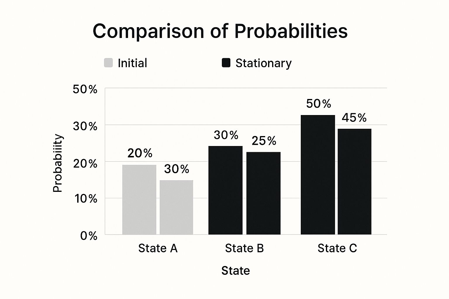
As you can see, after an initial "burn-in" period, the samples generated by the MCMC algorithm start to genuinely reflect the true underlying probabilities of the system we're modeling.

Gibbs Sampling: A Team of Specialists

Gibbs Sampling is another cornerstone MCMC algorithm, but it tackles the problem from a completely different angle. It's especially handy for problems that have multiple dimensions or parameters.

Instead of a single hiker, imagine you have a team of specialists trying to solve a complex puzzle. Each specialist is an expert on just one piece of the puzzle, but here's the catch: their decision depends entirely on the current state of all the other pieces.

Gibbs Sampling works in a similar "one-at-a-time" fashion:

1. It starts with an initial guess for all parameters.
2. It then samples a new value for the first parameter, keeping all the others fixed.
3. Next, it samples a new value for the second parameter, this time using the newly updated first parameter and the fixed values for the rest.
4. This process continues, cycling through each parameter one by one, updating it based on the current state of all the others.

This method cleverly breaks a complex, high-dimensional problem down into a series of much simpler, one-dimensional problems. Each individual step is far easier to solve, and by iterating through all the parameters repeatedly, the system as a whole gradually converges to the target distribution.

Metropolis-Hastings vs. Gibbs Sampling: A Quick Comparison

So, when should you use one over the other? The choice often boils down to the specific structure of your problem. This table breaks down the key differences to help you decide.

Characteristic	Metropolis-Hastings	Gibbs Sampling
Generality	Very general; works for almost any target distribution.	More specialized; requires sampling from full conditional distributions.
Proposal Distribution	Requires you to choose and tune a proposal distribution.	No proposal distribution needed; it's built-in.
Ease of Use	Can be difficult to tune the proposal for good performance.	Can be much easier and more "auto-magical" if conditionals are known.
Performance	Can be slow if the proposal is poor or parameters are correlated.	Very efficient if conditionals are easy to sample from.
Correlation Issues	Can handle correlated parameters, but might mix slowly.	Can get stuck and mix very slowly if parameters are highly correlated.

Both algorithms have their place. M-H is your reliable multitool, while Gibbs Sampling is the high-performance specialist you bring in when the conditions are just right.

Which One Should I Use?

Let's boil it down to some practical advice.

• Metropolis-Hastings is the generalist. It works even when you can't easily sample directly from the conditional distributions. The big catch is that its performance hinges on choosing a good proposal distribution. A bad choice is like our hiker taking steps that are either too tiny to get anywhere or too massive to ever be accepted. Tuning this is key to managing the bias-variance tradeoff in your model's sampling.

• Gibbs Sampling is the specialist. It absolutely shines when the conditional distributions for each parameter are known and easy to sample from. Since it doesn't need a hand-tuned proposal distribution, it can feel almost magical in its efficiency when it's applicable. The downside? If your parameters are highly correlated, Gibbs sampling can mix painfully slowly, like a team of specialists who can't make progress because their decisions are all too tightly interlocked.

Actionable Insight: Start with a general-purpose sampler like Metropolis-Hastings (or its modern variant, NUTS, found in libraries like PyMC). If your chain mixes poorly (i.e., fails convergence checks), investigate your model's structure. If it has known conditional distributions, switching to Gibbs Sampling for some parameters can dramatically improve efficiency.

Understanding these core engines is crucial for anyone looking to apply MCMC (Markov Chain Monte Carlo) in the real world. They aren't black boxes; they're structured, logical processes designed to navigate uncertainty. Once you grasp their internal logic, you gain the power to choose the right tool for the job and diagnose what's going wrong when your chains don't converge.

Building Your First Bayesian Model with MCMC

Okay, the theory is important, but let's be honest—the real learning happens when you get your hands dirty. It's time to move past the abstract ideas and build our first Bayesian model using an MCMC Markov Chain Monte Carlo approach. We'll walk through a common data science problem from start to finish.

Our example will tackle a classic business scenario: predicting product sales based on advertising spend. Instead of just finding a single "best-fit" line, the Bayesian method gives us something much richer: a full probability distribution for our model's parameters. This means we don't just get one answer. We get the entire range of plausible outcomes and a clear measure of the uncertainty in our predictions.

To make this happen, we'll use PyMC, a powerful and surprisingly intuitive Python library for probabilistic programming. PyMC does the heavy lifting, running complex sampling algorithms (like Metropolis-Hastings or its more advanced cousin, NUTS) behind the scenes. This frees us up to focus on what matters: the logic of our model.

This is the official logo for the PyMC project, a key tool in the modern data scientist's MCMC toolkit.

The library’s clean syntax and tight integration with the Python data science world make it a fantastic choice for putting MCMC to work on real problems.

Setting Up the Problem and Data

First things first, we need data. Let's pretend we've gathered sales and advertising data from 50 different markets. For each one, we have the total ad budget (in thousands of dollars) and the total sales (in thousands of units).

Our goal is to model the relationship between ad_spend and sales. A simple linear regression feels like a natural starting point. You probably remember the equation for a line:

sales = β * ad_spend + α + ε

• α (alpha) is the intercept: this represents our baseline sales if we spent zero on advertising.
• β (beta) is the slope: this tells us how much sales increase for every extra thousand dollars we spend.
• ε (epsilon) is the error term: this captures all the random noise and real-world variability our model can't explain.

In a traditional (frequentist) regression, the goal is to find the single best values for α and β. But we're thinking like Bayesians now. With an MCMC Markov Chain Monte Carlo approach, we’re going to find their entire posterior distributions instead.

Defining the Bayesian Model with Priors

This is where the Bayesian mindset really kicks in. Before we even let our model see the data, we have to define our initial beliefs about the parameters. These beliefs are called priors. Think of priors as a way of giving the model some gentle guidance on what we consider reasonable values for alpha, beta, and the error.

We'll set what are known as "weakly informative" priors. We don't want to strong-arm the model, just provide some sensible starting points.

• For α (intercept): We'll assume it follows a Normal distribution centered around the average sales in our dataset. That’s a pretty safe bet for a starting point.
• For β (slope): We can also assume this follows a Normal distribution, but we'll center it at zero. We’re being neutral—we don't know if spending more on ads will help or hurt, so we'll let the data decide. We'll give it a wide standard deviation to let the data pull it wherever it needs to go.
• For ε (error): The standard deviation of the error (often called sigma) has to be positive. A Half-Normal distribution is a common and solid choice for this.

Actionable Insight: Choosing priors is a modeling decision. If you have strong domain knowledge (e.g., "I am certain the slope, β, cannot be negative"), incorporate it into your prior. This can lead to more stable and faster-converging models. Start with weakly informative priors if you are unsure.

Here’s what this model looks like in Python using PyMC. Notice how the code is almost a direct translation of the statistical model we just described.

import pymc as pm
import pandas as pd
import numpy as np

# Assume 'data' is a pandas DataFrame with 'ad_spend' and 'sales' columns
# For a practical example, let's create some sample data:
np.random.seed(42)
ad_spend = np.random.rand(50) * 10
sales = 2.5 * ad_spend + 5 + np.random.normal(0, 2, 50)
data = pd.DataFrame({'ad_spend': ad_spend, 'sales': sales})

with pm.Model() as sales_model:
    # 1. Define Priors for our parameters
    alpha = pm.Normal('alpha', mu=data['sales'].mean(), sigma=10)
    beta = pm.Normal('beta', mu=0, sigma=10)
    sigma = pm.HalfNormal('sigma', sigma=10)

    # 2. Define the Expected Value (our linear equation)
    mu = alpha + beta * data['ad_spend']

    # 3. Define the Likelihood (how the data is distributed)
    sales_likelihood = pm.Normal('sales_likelihood', mu=mu, sigma=sigma, observed=data['sales'])

Running the MCMC Sampler

With the model fully specified, it's time to run the sampler. This is where the magic happens. PyMC will unleash its MCMC algorithm to explore the parameter space, generating thousands of samples for alpha, beta, and sigma from the posterior distribution.

with sales_model:
    # 4. Run the MCMC sampler to generate posterior samples
    trace = pm.sample(2000, tune=1000, cores=1)

The pm.sample() function tells the sampler to generate 2000 samples for each chain, but only after an initial "tuning" (or burn-in) period of 1000 samples. These first steps are discarded because they represent the sampler's initial wandering as it tries to find the high-probability zone. The 2000 samples that remain are what we'll use for our analysis. This whole process is quite a bit more involved than what you'd see in simpler time-series models; for a different take on forecasting, you can read our guide on ARIMA models in Python.

Once the sampling is done, the trace object holds our results. It doesn't contain a single number for beta. Instead, it holds 2000 different plausible values for beta, where each one is a draw from the posterior distribution. This collection of samples is the answer—a rich, nuanced picture of the relationship between ad spend and sales, complete with built-in uncertainty.

How to Know if Your MCMC Model Is Reliable

Running an MCMC simulation is one thing; knowing you can actually trust its output is a completely different beast. Just because your code runs to completion doesn't mean the results are meaningful. This brings us to the most critical step in the process: checking for convergence. It's a non-negotiable part of any serious MCMC Markov Chain Monte Carlo analysis.

Let's go back to our hiker trying to map a foggy mountain range. If they only spend a few minutes on one small hill, their map of the entire range will be wildly inaccurate. To create a reliable map, they need to wander long enough and cover enough ground to be certain they've explored the whole terrain and found all the important peaks.

This is precisely what convergence diagnostics help us figure out. Has our sampler run long enough to forget its random starting point (the "burn-in" phase) and truly explore the high-probability areas of our posterior distribution? If we don't confirm this, our conclusions might be based on a fleeting, localized glimpse rather than the true, stable picture.

Visual Checks with Trace Plots

Your first line of defense—and the most intuitive check—is to simply look at the output. A trace plot is a simple line graph showing the value of a parameter at each step of the Markov chain. What you're hoping to see is something that looks like a "fuzzy caterpillar"—a stationary, horizontal band of noise with no obvious trends.

A healthy trace plot is a great sign that the chain is "mixing" well. It's zipping around the most likely values and not getting stuck in any single spot. This quick visual check is your best initial guard against unreliable results.

But looks can sometimes be deceiving, so you also need to know what red flags to watch out for.

• Slow, snake-like trends: If the plot shows a slow, winding path either up or down, your chain hasn't converged. It's still in the burn-in phase, trying to locate the main body of the probability mass. The fix? Run it for longer.
• Getting stuck: If the line flatlines at a single value for long periods, your sampler isn't exploring the space properly. This often points to a deeper issue with your model's setup or how its parameters are related.

Actionable Insight: A healthy trace plot for a parameter should look like random noise centered around a stable mean. It should not show any long-term trends, drifts, or periods where the sampler gets stuck. This is the visual signature of a converged MCMC chain. If you see poor mixing, your immediate actions should be: 1) Increase the number of tuning/burn-in steps. 2) Check if your priors are too vague. 3) Simplify your model if possible.

Quantitative Checks with the Gelman-Rubin Statistic

While trace plots are indispensable, you can't just eyeball it. We need a more formal, numbers-based measure of convergence. This is where the Gelman-Rubin statistic, almost always called R-hat (or R̂), comes in. It's the gold standard for diagnosing MCMC convergence.

The idea behind R-hat is actually pretty simple. It works by comparing the variance within a single Markov chain to the variance between several different chains (which you start from different random points). If all the chains have truly converged, the variation within each one should look just like the variation between them.

Here's how to interpret the R-hat value:

• R-hat ≈ 1.0: This is what you want to see. It means all your chains have settled on the same distribution. A value below 1.01 is generally considered solid proof that your model is reliable.
• R-hat > 1.1: This is a major warning sign. It tells you the chains haven't agreed on an answer yet, and the variance between them is still way bigger than the variance within them. Your results simply aren't trustworthy at this point.

Running these diagnostics isn't a one-and-done task; it's a continuous part of the modeling workflow. Rigorously checking model performance is a cornerstone of responsible data science, a topic we cover in our guide to effective machine learning model monitoring. By combining visual checks with quantitative tests like R-hat, you can build real confidence that your MCMC Markov Chain Monte Carlo results aren't just numbers, but genuine, reliable insights.

Real-World Applications of MCMC in Modern AI

Any complex algorithm is only as good as the real problems it can solve. This is where MCMC (Markov Chain Monte Carlo) truly proves its worth, bridging the gap from abstract theory to tangible impact across a surprisingly diverse set of fields. Its real power lies in its unique ability to navigate and make sense of uncertainty, making it essential for challenges that are simply too messy for direct calculation.

MCMC acts as the inference engine for everything from cutting-edge AI to the life sciences. By generating samples from complex posterior distributions, it empowers researchers and data scientists to see the full spectrum of possibilities, rather than settling for a single, often misleading, best guess. This is a game-changer wherever uncertainty isn't just a nuisance—it's a core feature of the problem.

Quantifying Uncertainty in AI and Machine Learning

In the AI world, MCMC is a cornerstone of Bayesian machine learning. One of its most critical jobs is training Bayesian Neural Networks (BNNs). A standard neural network gives you a single point prediction, but a BNN provides a full distribution of possible outcomes. This gives you a built-in measure of the model's confidence in its own answers. MCMC is the workhorse that estimates the posterior distributions for the network's weights, effectively transforming a "black box" into a transparent, uncertainty-aware model.

It also plays a huge role in Natural Language Processing (NLP). For instance, topic modeling algorithms like Latent Dirichlet Allocation (LDA) lean heavily on MCMC, particularly Gibbs sampling. When you use LDA to uncover abstract topics from a massive collection of documents, it's MCMC that helps the algorithm explore the vast landscape of possible word-topic combinations, eventually settling on a coherent model of the underlying themes.

Actionable Insight: The real value of MCMC in AI is that it reframes the question from "What is the answer?" to "What is the entire range of plausible answers?" This shift is fundamental for building safer and more reliable AI, especially in high-stakes fields like healthcare and finance where understanding the scope of uncertainty is non-negotiable.

Powering Insights Across Scientific Disciplines

MCMC's influence stretches far beyond the tech industry. Its knack for solving thorny inference problems has made it an indispensable tool across a host of scientific and commercial domains.

• Financial Risk Modeling: Financial institutions use MCMC to model extreme market events and calculate crucial metrics like Value at Risk (VaR). Practical Example: A bank can simulate thousands of possible futures for its loan portfolio, using MCMC to understand the probability of different default rates under various economic stresses, leading to better capital allocation.

• Epidemiological Forecasting: When public health crises hit, epidemiologists turn to MCMC to model the spread of infectious diseases. These models are packed with uncertain variables—like transmission rates or recovery times—and MCMC is what allows them to estimate these parameters and generate a full range of likely outbreak scenarios, which helps guide public policy.

• Computational Biology and Genetics: In genetics, MCMC is used to piece together evolutionary history by building phylogenetic trees. Given DNA sequences from different species, MCMC algorithms explore the astronomical number of possible evolutionary trees, sampling those that best explain the genetic differences we observe today. The result isn't just one tree, but a whole distribution of plausible evolutionary stories.

From forecasting financial meltdowns to revealing the hidden topics in millions of documents, the practical applications of MCMC (Markov Chain Monte Carlo) are both broad and deep. As we’ve discussed in our Datanizant guide on building robust machine learning systems, methods that can gracefully handle complexity and uncertainty are what truly drive progress.

Common Questions About MCMC

Once you start working with MCMC Markov Chain Monte Carlo methods, a few practical questions almost always pop up. Getting good, straightforward answers can be the difference between a successful model and a lot of frustration. Let's dig into some of the most common ones.

How Many Samples Do I Need for My MCMC Simulation?

This is the classic "it depends" question, but we can definitely establish some solid rules of thumb. The real goal isn't just to rack up a huge number of samples; it's to get a large effective sample size. It all comes down to balancing the computational work with the accuracy you need.

A typical simulation runs in two main phases:

• Burn-in Period: Think of these as the warm-up laps. You discard these initial samples because the chain needs a moment to forget its random starting point and find the high-probability sweet spot. A burn-in of 1,000 to 5,000 samples is a common starting point, but you always want to confirm this by looking at your trace plots.
• Sampling Period: After the burn-in, you start collecting the samples that will actually inform your analysis. For many problems, running at least 10,000 samples post-burn-in is a good place to start. If you're working with a particularly complex model, you might need way more to get a stable posterior distribution.

Actionable Insight: Instead of picking a magic number, monitor convergence. Start with a moderate number of samples (e.g., 2,000 burn-in, 5,000 collected). Check your trace plots and R-hat values. If convergence is not achieved or posterior distributions look rough, double the number of samples and check again. Repeat until your results are stable.

What Are Common Pitfalls When Using MCMC?

Even seasoned pros can stumble into a few common traps with MCMC. Just knowing what they are is the first step to sidestepping them and making sure your model is sound.

Here are three frequent mistakes to watch out for:

1. Poor Mixing: This is what happens when your sampler gets stuck in one little corner of the parameter space and doesn't explore the whole landscape. You'll see this in trace plots that look "sticky" or snake-like instead of like a nice, fuzzy caterpillar. Often, you can fix this by re-parameterizing your model or switching to a more advanced sampler.
2. Bad Priors: Your choice of priors can make or break your model. Priors that are too confident (overly narrow) can steamroll your data, preventing it from telling its own story. On the other hand, priors that are completely uninformative can leave your sampler wandering aimlessly, struggling to converge. The sweet spot is usually "weakly informative" priors that give a gentle nudge in the right direction without dominating the outcome.
3. Misinterpreting Convergence: A quick glance at a single trace plot just isn't enough. It's absolutely critical to use quantitative diagnostics like the R-hat statistic. A high R-hat value is a big red flag that your chains haven't converged to the same distribution, meaning your results can't be trusted.

Is MCMC Still Relevant in the Age of Deep Learning?

Absolutely. It's a common mistake to view MCMC and deep learning as competitors. In reality, they are incredibly complementary, with each one picking up where the other leaves off.

Deep learning models are fantastic at approximating functions and finding intricate patterns in massive datasets. The catch? Most traditional deep learning models give you a single point prediction, with no real sense of their own uncertainty.

This is exactly where MCMC Markov Chain Monte Carlo shines. Its entire reason for being is to quantify uncertainty. The growing field of Bayesian deep learning brings these two worlds together, using MCMC or similar methods to put error bars on a neural network's predictions. For anyone aiming for true machine learning mastery, knowing how to blend probabilistic methods like MCMC is a vital skill for building more robust and trustworthy AI systems.

---

At DATA-NIZANT, we are committed to providing expert-led analysis and in-depth guides on the most important topics in AI, machine learning, and data science. To continue building your expertise, explore our extensive resources at https://www.datanizant.com.