Striking the Balance Between Underfitting and Overfitting in Machine Learning Models: Bias Variance Tradeoff: Mastering Model Balance

Why Your Models Miss The Mark (And How To Fix It / Mastering Model Balance)

Imagine you’re coaching a darts player. If all their throws cluster together on the wall, but far from the bullseye, they have a bias. Their technique has a systematic flaw that makes them consistently miss in the same way. Now, picture another player whose throws are scattered all over the board—some are close, some are way off, but there’s no consistency. This wild spread is variance. This exact same challenge affects every machine learning model you build, often determining if it succeeds or fails in the real world.

This fundamental tension between these two errors is called the bias-variance tradeoff. It’s more than just a theoretical idea; it’s a practical hurdle that distinguishes effective data scientists from those whose models don’t perform well when deployed. A model with high bias is too simplistic; it makes broad assumptions and fails to see the real patterns in the data. On the other hand, a model with high variance is too complex; it learns the training data, including its random noise, so perfectly that it can’t make reliable predictions on new, unseen data.

The Two Faces of Model Error: Bias and Variance

At its heart, the bias-variance tradeoff is about finding a sweet spot. You can’t just get rid of one error without impacting the other. If you make a model more flexible to reduce its bias, you will often increase its variance. Conversely, simplifying a model to lower its variance might increase its bias, causing it to overlook key relationships. It’s a delicate balancing act that requires careful tuning.

The following graphic perfectly illustrates the relationship between these two sources of error.

This visual shows four scenarios combining different levels of bias and variance. The ideal outcome is the top-right quadrant: low bias and low variance, where predictions are both accurate and consistent.

The bias–variance tradeoff is a core principle explaining this tension. To put it simply:

• Bias is an error from overly simple assumptions in your algorithm. It leads to a model that underfits, meaning it misses the true connections within the data.
• Variance is an error from being too sensitive to minor fluctuations in the training data. This causes the model to overfit, performing poorly on any new data it hasn’t seen before.

For a deeper dive into this foundational concept, check out the detailed overview of the bias-variance tradeoff on Wikipedia.

Real-World Consequences of Imbalance

Failing to manage this tradeoff can have serious consequences. Let’s look at two practical examples:

• High Bias (Underfitting): A bank builds a loan approval model. If the model is too simple (high bias), it might learn only one rule, like “approve loans only for high-income applicants.” This model would ignore other vital factors like credit history or debt levels, causing it to unfairly reject many qualified applicants and potentially approve risky ones. Its predictions are too blunt to be useful.

• High Variance (Overfitting): An e-commerce site creates a recommendation engine. If the model is too complex (high variance), it might learn that a customer who bought a red shirt on a Friday is only interested in red items on Fridays. The model has essentially memorized the noise in the training data. When presented with new customer behavior, its recommendations will be bizarre and irrelevant, hurting the user experience.

Recognizing these issues early is key. A model that performs poorly on both your training and test data is likely suffering from high bias. In contrast, a model that achieves near-perfect results on the training set but fails badly on the test set is a classic case of high variance. Learning how to diagnose and correct this imbalance is what separates models that just work on paper from models that deliver real-world value.

The Hidden Math That Controls Model Performance

To truly master the bias-variance tradeoff, we need to peek behind the curtain and understand the mathematical forces at play. Every prediction error your model makes can be broken down into three distinct, competing components. This idea is known as error decomposition, and it shows that the total expected error is defined by a specific formula:

Total Error = Bias² + Variance + Irreducible Error

Getting a handle on these three parts is the key to diagnosing and improving your models with precision. Let’s explore each one.

The Three Components of Prediction Error

Think of these components as three dials you, the data scientist, must carefully tune. Getting the balance right is what separates a good model from a great one.

• Bias² (Bias Squared): This term represents the error from your model’s simplifying assumptions. A simple linear regression model trying to capture a complex, curved trend will have high bias because its core assumption (a straight line) is fundamentally wrong for the data. Squaring the bias term penalizes larger errors more heavily, highlighting just how far off your model’s average prediction is from the real value.

• Variance: This component measures how sensitive your model is to the specific training data it learned from. A very flexible model, like a deep neural network or a high-degree polynomial, might fit the training data perfectly but give wildly different predictions if trained on a slightly different sample. This instability is variance. Some models, like those discussed in our guide on Gaussian process machine learning, are designed to inherently manage this kind of uncertainty.

• Irreducible Error: This is the baseline noise that no model can ever get rid of, no matter how powerful it is. It represents the natural randomness within the data itself. For instance, when predicting house prices, there will always be unmeasurable factors, like a buyer’s personal taste, that create a floor on how accurate any prediction can possibly be.

This infographic helps visualize a model with high bias. The model is too simple and fails to capture the underlying pattern in the data, a classic case of underfitting.

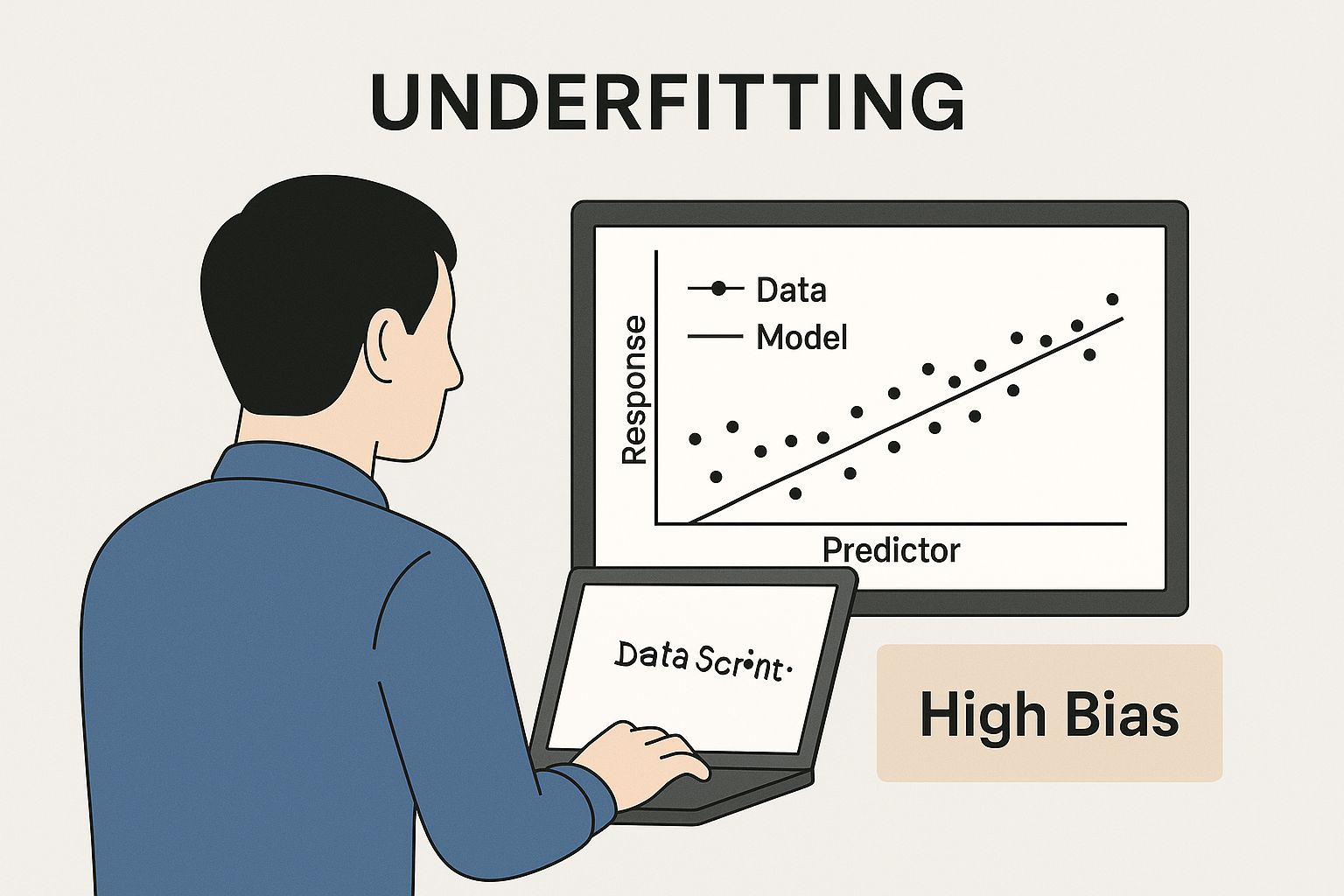
The straight line in the chart clearly misses the curved trend of the data points, illustrating a model that isn’t complex enough for the job.

The Intricate Dance of Model Complexity

The relationship between these components is what makes the bias-variance tradeoff so tricky. As you increase a model’s complexity to lower its bias, you almost always increase its variance. For example, switching from a simple linear model to a complex decision tree lets the model capture more detailed patterns, which reduces bias. However, this new flexibility also makes it more likely to “memorize” the noise in the training data, which raises its variance.

To illustrate how these components interact as a model becomes more complex, consider the following table. It shows the typical relationship between complexity, bias, variance, and the overall error.

Model Complexity	Bias Level	Variance Level	Total Error	Risk Factor
Low	High	Low	High, dominated by bias	Underfitting
Medium	Medium	Medium	Low, at or near the optimal point	Balanced
High	Low	High	High, dominated by variance	Overfitting
Very High	Very Low	Very High	Very high, model is essentially memorizing noise	Severe Overfitting

This table highlights the central challenge: finding the sweet spot. The goal is to find a level of model complexity where the sum of bias squared, variance, and irreducible error is at its lowest. You can explore the foundational principles in more detail by reviewing this comprehensive overview of the bias-variance tradeoff. This mathematical reality guides every decision in machine learning, from choosing an algorithm to tuning its hyperparameters.

Diagnosing Your Model’s Real Problems

To truly master the bias-variance tradeoff, you need to stop guessing what’s wrong with your model and start diagnosing its issues like a detective. Simply looking at final accuracy scores is like trying to fix an engine without ever popping the hood. Skilled data scientists use a systematic approach to pinpoint the root cause of model errors, and learning curves are a fundamental tool in this diagnostic process.

Interpreting Learning Curves

Learning curves are charts that plot a model’s performance on both the training and validation data as the amount of training data increases. They tell a story about how your model learns, revealing its strengths and, more importantly, its weaknesses.

• High Bias (Underfitting): Imagine the learning curves for both training and validation error are high and have flattened out close to each other. This is a classic sign of underfitting. The model is too simple to grasp the underlying patterns in the data. No matter how much more data you feed it, the error won’t improve because the model’s core assumptions are flawed.

• High Variance (Overfitting): Now, picture a large and persistent gap between the training and validation error. The training error is incredibly low, but the validation error is much higher. This signals overfitting. The model has essentially memorized the noise and specific details of the training set, failing to generalize to new, unseen data. In this case, adding more data is often a great strategy to help the model learn the true signal.

A Practical Diagnostic Checklist

It’s surprisingly easy to misdiagnose a model’s performance issues. For instance, what seems like overfitting in a complex algorithm like a Decision Tree might just be its natural tendency toward high variance. To see how different algorithms manage this, you can explore our detailed comparison of a decision tree vs. a random forest, where ensemble techniques are specifically used to reduce variance.

To help you systematically determine if your model is struggling with bias or variance, use the following checklist. It provides clear indicators and recommended actions for each symptom.

Symptom	High Bias Indicator	High Variance Indicator	Recommended Action
Performance on Training Data	Poor performance (high error)	Excellent performance (low error)	Compare training and validation performance to establish a baseline.
Performance on Validation Data	Poor performance, similar to training error	Poor performance, much worse than training error	Assess the gap between the two error rates to spot generalization issues.
Learning Curve Shape	Training and validation curves plateau at a high error	Large, persistent gap between low training and high validation curves	Identify the convergence point and the size of the error gap.
Effect of More Data	Little to no improvement	Performance improves as the gap narrows	Use learning curves to project whether collecting more data is worthwhile.
Model Complexity	Often a simple model (e.g., linear regression)	Often a complex model (e.g., deep neural network)	Consider choosing a different model architecture based on the diagnosis.

By using these diagnostic tools, you move from guesswork to informed, data-driven decisions. You can confidently decide whether your model needs more data, increased complexity, or a completely new architectural approach, saving you valuable time and resources. This structured process is the key to effectively navigating the bias-variance tradeoff.

Regularization Techniques That Actually Move The Needle

Regularization isn’t just a theoretical concept; it’s a practical toolkit for managing the bias-variance tradeoff when your model’s performance really counts. When you have a model with high variance (a classic case of overfitting), the goal is to introduce a small, controlled amount of bias to help it generalize better to new, unseen data. Think of it as applying a “penalty” for too much complexity, which encourages the model to focus on the most important signals instead of getting lost in the noise.

This process involves tweaking a hyperparameter—usually called lambda (λ) or alpha (α)—that sets the strength of this penalty. If the penalty is too weak, it might not be enough to fix the variance problem. If it’s too strong, you might oversimplify the model and end up with high bias. The sweet spot is what we’re after. Studies on the bias-variance tradeoff have shown how significant this can be. For instance, in ridge regression, as the regularization parameter λ increases, model variance can drop by more than 50%, often with only a minor increase in bias. You can explore an empirical analysis of this effect to see the numbers behind this phenomenon.

L1 vs. L2: Choosing Your Weapon

Two of the most popular and useful regularization methods are L1 (Lasso) and L2 (Ridge) regression. While they both aim to curb model complexity, they achieve it in different ways, making them suitable for different kinds of problems.

• L2 Regularization (Ridge Regression): This technique adds a penalty based on the squared value of the model’s coefficients. It works by shrinking large, less important coefficients closer to zero, but it rarely eliminates them completely. Ridge is fantastic for handling multicollinearity (when your features are highly correlated) and serves as a solid default choice for cutting down variance without being too aggressive about removing features. It effectively smooths out the model’s predictions.

• L1 Regularization (Lasso Regression): Lasso, which stands for Least Absolute Shrinkage and Selection Operator, adds a penalty based on the absolute value of the coefficients. This approach has a unique and powerful side effect: it can shrink some coefficients all the way to zero. This makes Lasso an excellent tool for automatic feature selection, simplifying your model by getting rid of irrelevant inputs. To see how this works in a real project, check out our guide on effective feature selection techniques.

Which One Should You Use?

The choice between Ridge and Lasso comes down to your primary goal. If you think all your features have some relevance and you just need to dial back overfitting, Ridge is usually the safer and more stable option. On the other hand, if you suspect that many features are just noise and you want a simpler, more interpretable model, Lasso is the clear winner.

Here’s a quick guide to help you decide:

Scenario	Recommended Technique	Why It Works
High variance and many features	L2 (Ridge)	Shrinks coefficients to reduce model sensitivity without removing potentially useful features.
Suspected irrelevant features	L1 (Lasso)	Performs automatic feature selection by forcing irrelevant feature coefficients to zero.
Need for a simpler, interpretable model	L1 (Lasso)	Creates a sparser model that is easier to explain to stakeholders.
Features are highly correlated	L2 (Ridge)	Handles multicollinearity better than Lasso, which might arbitrarily pick one feature over another.

For situations where you want the benefits of both, there’s Elastic Net regularization. It combines the L1 and L2 penalties into one. This allows you to perform feature selection while also managing multicollinearity, giving you a flexible solution for complex datasets where the best path forward isn’t obvious.

How Industry Leaders Handle The Tradeoff

The theoretical dance of the bias-variance tradeoff shifts when it meets real-world business problems. There is no single “correct” balance; instead, the ideal point on the spectrum is a strategic choice. This choice is defined by an industry’s specific goals, the nature of its data, and how much it can tolerate different kinds of errors. Leaders across various sectors approach this challenge differently, offering valuable lessons for any data scientist.

High-Stakes vs. High-Volume Applications

Let’s compare financial fraud detection with e-commerce recommendations. A bank building a fraud model simply cannot afford many false negatives (a sign of high bias). Missing even one fraudulent transaction could result in millions of dollars in losses. To avoid this, they would rather accept some false positives (higher variance), like flagging a legitimate purchase for review, than let any actual fraud go undetected. Their models are therefore intentionally complex and tuned for high sensitivity.

On the other hand, an e-commerce giant recommending products can live with a bit more error. An imperfect recommendation is a minor annoyance, not a financial disaster. The primary goal is to drive broad user engagement. They might opt for models that are slightly biased toward popular items but are less likely to make bizarre, overfitted suggestions. This strategy ensures a consistently decent experience for millions of users, even if it’s not perfectly personalized every time.

Navigating Data Dimensionality

The structure of the data itself plays a huge role in managing the tradeoff. Fields like computer vision and genomics deal with extremely high-dimensional data, where the number of features (like pixels or genes) can dwarf the number of samples (images or patients). In these cases, a model can easily achieve low bias but then suffer from extreme variance, effectively just memorizing the training data.

Here, regularization becomes a critical tool, not just a “nice-to-have.” By systematically penalizing model complexity, teams can pull the variance back into a reasonable range. For example, carefully tuning a regularization parameter (λ) to minimize cross-validation error can reduce a model’s total error by up to 30% compared to its unregularized counterpart. You can discover more about the statistical analysis of bias and variance to see the math behind these gains.

Conversely, Natural Language Processing (NLP) often involves sparse text data. A model trying to predict sentiment from customer reviews might have high bias if it only learns from a handful of common positive or negative words. The focus here shifts to creating richer features and using more flexible models to capture subtle meanings, which in turn requires careful management of the resulting increase in variance.

The table below shows how different needs lead to different approaches for the bias-variance tradeoff.

Industry/Application	Primary Concern	Typical Model Preference	Key Strategy
Financial Fraud Detection	Avoiding false negatives (missed fraud)	Low Bias, Higher Variance	Build highly sensitive, complex models.
E-commerce Recommendations	User engagement and satisfaction	Balanced Bias-Variance	Optimize for general performance at scale.
Computer Vision/Genomics	Overfitting due to high dimensionality	High Bias (controlled), Low Variance	Employ strong regularization and feature reduction.
Healthcare Diagnostics	High accuracy and reliability	Low Bias, Low Variance	Use ensemble methods and rigorous validation.

Ultimately, the most successful teams don’t search for a generic “best” model. They strategically align their bias-variance tradeoff approach with their specific business context, understanding that the perfect balance is always relative to the problem they are trying to solve.

Advanced Strategies Beyond Basic Regularization

While regularization is a fantastic tool for tuning a single model, truly mastering the bias-variance tradeoff often means looking beyond one model’s limitations. The most effective machine learning practitioners use advanced methods that change the error landscape entirely, often tackling both bias and variance at the same time. These strategies are what separate a good model from a great one, leading to more robust and accurate performance on messy, real-world data.

One of the most powerful approaches is using ensemble methods. Instead of putting all your faith in a single model, you combine the predictions from several models to get a much stronger result. It’s a clever way to balance the bias-variance equation.

Ensemble Methods: The Power of Collaboration

Think of it like asking a group of experts for their opinion instead of just one. Ensemble methods pool the “knowledge” of multiple models to arrive at a better conclusion. The two main approaches, bagging and boosting, each target a different side of the error problem.

• Bagging (Bootstrap Aggregating): This technique is designed to reduce high variance. Imagine you have a model that’s a bit unstable—it changes wildly with small shifts in the training data. Bagging smooths out this instability. It works by creating many different random subsets of your training data (a process called bootstrapping) and training a model on each one. The final prediction is simply the average of all the individual model predictions. A classic example is the Random Forest algorithm, which builds hundreds of decision trees on different data samples. Because each tree sees a slightly different view of the data, their individual errors tend to cancel each other out, resulting in a much more stable and reliable final model.

• Boosting: In contrast, boosting is all about reducing high bias. This method builds models one after another, in a sequence. Each new model is specifically trained to fix the mistakes its predecessor made. Algorithms like AdaBoost and Gradient Boosting give more attention to the data points that previous models got wrong, forcing the system to learn the more difficult and complex patterns in the data. This process turns a collection of “weak learners” (simple, high-bias models) into a single, powerful “strong learner” with low bias.

Advanced Cross-Validation and Optimization

Even with the best algorithms, how you test and tune your model matters immensely. A frequent mistake is accidentally overfitting to the validation set. If you keep tweaking hyperparameters and picking the combination that works best on your single validation set, you might just be finding the settings that got lucky on that specific slice of data, not the ones that will generalize well to new, unseen data.

To guard against this, you can use more robust validation techniques like nested cross-validation. This method uses two loops: an outer loop to evaluate the final model’s true performance and an inner loop dedicated to finding the best hyperparameters. This strict separation ensures your performance metrics reflect the model’s ability to generalize, not just its ability to fit one particular validation split.

Furthermore, searching for the best hyperparameters can take a lot of time and computational power. Instead of a brute-force grid search that tries every possible combination, Bayesian optimization offers a smarter path. It builds a probability model of the loss function and uses it to intelligently select the most promising hyperparameters to try next. This approach often discovers optimal settings in far fewer attempts, saving you significant time and compute resources while you navigate the delicate bias-variance tradeoff.

Your Bias-Variance Mastery Roadmap

Moving from theory to practice is where you truly forge expertise in the bias-variance tradeoff. This roadmap gives you a repeatable framework to diagnose issues, apply solutions, and measure your progress. It’s all about creating a disciplined workflow that turns abstract concepts into real-world results.

A Three-Step Diagnostic Workflow

Seasoned data scientists don’t guess; they diagnose. You can follow this same proven process to systematically find and fix imbalances in your models.

1. Initial Diagnosis with Learning Curves: The first step is to always plot your learning curves. Do the training and validation error curves meet up at a high error rate? This is a classic sign of high bias. Or, is there a wide, stubborn gap between a low training error and a much higher validation error? That’s the textbook definition of high variance. This initial check tells you exactly which problem you need to solve.
2. Targeted Solution Application: With a clear diagnosis, you can now pick the right tool for the job.
   • For High Bias (Underfitting): Your goal is to increase the model’s complexity. You could try a more powerful algorithm (like moving from linear regression to a gradient-boosted tree), create more insightful features through feature engineering, or dial back the regularization strength.
   • For High Variance (Overfitting): Here, you need to either decrease model complexity or get more data. Try increasing the regularization strength (by tuning L1 or L2), adding dropout layers, using early stopping, or gathering more training examples to help the model learn the general patterns.
3. Validate and Iterate: After applying a solution, it’s time to re-evaluate your model with a solid cross-validation strategy. Did the total error go down? Did the shape of the learning curves improve? Keeping detailed records of each experiment is essential. Note the model type, hyperparameters, and the performance metrics you achieved to track what works and what doesn’t.

A Framework for Continuous Improvement

Mastering the bias-variance tradeoff is an ongoing practice, not a one-and-done task. You can use this table as a handy decision-making guide for your projects.

Stage	Goal	Key Actions	Metrics to Monitor
1. Problem Framing	Define error tolerance	Figure out the business impact of false positives versus false negatives.	Cost of error, stakeholder priorities.
2. Diagnosis	Identify the dominant error	Analyze learning curves and compare performance on train/validation sets.	Training Error, Validation Error, Gap Size.
3. Solution Selection	Choose the right technique	Apply regularization, change model complexity, or use ensemble methods.	Cross-Validation Score, Hyperparameter values.
4. Measurement	Quantify the improvement	Compare cross-validation scores before and after making changes.	Change in Mean Squared Error (MSE), F1-Score.

This structured process changes the bias-variance tradeoff from a frustrating hurdle into a clear opportunity for optimization. It provides a reliable path to building models that are not just theoretically sound but also effective in practice.

Ready to put these ideas into action and explore more advanced machine learning topics? Visit DATA-NIZANT at https://www.datanizant.com to find in-depth articles, expert analyses, and practical guides built for data professionals.