This blog was originally written during the height of ARIMA’s adoption in Python-based forecasting workflows. Backdated to February 18, 2016, to reflect its historical significance.

ARIMA – AutoRegressive (AR) Integrated (I) Moving Average (MA)

• Gravatar

Breaking Down ARIMA Components (Without The Confusion)

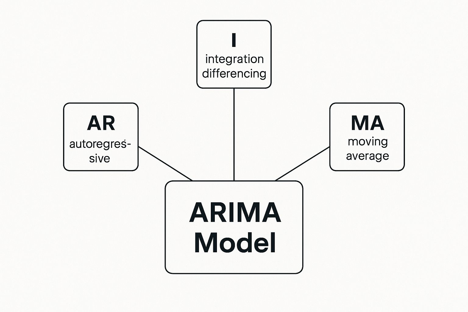
The infographic above provides a visual representation of how the core components of an ARIMA model work together. The AR, I, and MA components, while distinct, are interconnected, creating a robust predictive model capable of handling the intricacies of time series data. Understanding this interplay is key to effectively utilizing ARIMA in Python.

Let’s explore each component in more detail.

AutoRegressive (AR)

The AutoRegressive (AR) component, represented by the p parameter, analyzes past values to predict future ones. Imagine trying to predict the price of gold tomorrow based on its price over the past few days. The p value indicates how many past periods are considered. A larger p value signifies the model incorporates more historical data.

Integrated (I)

Time series data often exhibits non-stationarity, where statistical properties change over time. This poses a challenge for accurate prediction. The Integrated (I) component, denoted by d, tackles this by differencing the data, essentially subtracting a previous value from the current one. This helps stabilize the data, making it more suitable for ARIMA modeling. The d value indicates the degree of differencing performed.

Moving Average (MA)

The Moving Average (MA) component, denoted by q, utilizes past forecast errors to refine future predictions. Think of it as adjusting predictions based on previous overestimations or underestimations. The q value indicates how many past forecast errors are incorporated.

To further illustrate the differences and functionalities of these components, let’s look at a comparison table.

The table below, “ARIMA Components Comparison”, provides a detailed breakdown of the AR, I, and MA components, outlining their functions and common applications.

Component	Function	Purpose	Common Applications
AR(p)	Uses past values to predict future values	Captures autocorrelation in the time series	Predicting stock prices, sales forecasting
I(d)	Differences the data to make it stationary	Removes trends and seasonality	Stabilizing economic data, removing trends in sensor readings
MA(q)	Uses past forecast errors to improve future predictions	Corrects for short-term fluctuations	Adjusting inventory levels, fine-tuning demand forecasts

As shown in the table, each component plays a unique role in making ARIMA a powerful forecasting tool. Understanding these roles is crucial for model selection and parameter tuning.

These three components – AR, I, and MA – are the fundamental building blocks of ARIMA models. ARIMA, a popular statistical method for analyzing and forecasting time series data, especially within Python, leverages these three components. The AutoRegressive (AR) component uses historical data to forecast future values; the Integrated (I) component addresses the presence of a unit root by making the data stationary; and the Moving Average (MA) component incorporates past prediction errors for improved forecasting. Implementing ARIMA models in Python is facilitated by libraries like statsmodels. This allows for efficient model creation and evaluation. A common application is forecasting gold prices over time using historical data to predict future trends. Research indicates ARIMA’s effectiveness in diverse fields like climate change modeling, where understanding historical weather patterns helps predict future conditions. Explore this topic further: Time series analysis with ARIMA models in Python

By grasping how these components interact, we can build effective ARIMA models for accurate time series forecasting. This knowledge is essential for selecting appropriate parameters and optimizing models for various forecasting scenarios.

Setting Up Your Python Environment (The Right Way)

A well-structured Python environment is essential for implementing ARIMA models effectively. A poorly configured setup can lead to errors and inaccurate results, hindering your analysis. This guide will walk you through setting up your environment correctly for a smooth modeling process.

Choosing the Right Datasets

ARIMA models require specific types of data. The model needs time series data, which is collected over time at consistent intervals. Examples of suitable datasets include historical stock prices, weather patterns, sales figures, and website traffic. Selecting a dataset with these temporal dependencies is the first crucial step.

Essential Python Libraries

Several Python libraries are key for ARIMA modeling. The core library is Statsmodels, which provides the functions for building and analyzing your models. Pandas offers powerful tools for data manipulation and time series handling, while NumPy provides numerical computation capabilities.

• Pandas: Essential for data cleaning, transformation, and time series manipulation.
• NumPy: NumPy arrays and functions are crucial for numerical operations.
• Statsmodels: The core library for implementing and analyzing ARIMA models in Python.

Data Structure and Preprocessing

Data structuring is often overlooked but is crucial for accurate ARIMA modeling. Your time series data should be formatted so Statsmodels can interpret it correctly. This typically means using a Pandas Series or DataFrame with a datetime index.

• Datetime Index: This allows the model to understand the temporal order of your data.
• Consistent Time Intervals: ARIMA expects consistent intervals between data points. Preprocess data with irregular intervals accordingly.
• Handling Missing Values: Address any missing data through imputation or removal before modeling, as missing values can impact accuracy.

Implementing an ARIMA model involves steps from dataset selection to parameter tuning. This includes using libraries like statsmodels and sklearn, loading the dataset into a pandas DataFrame with correct date parsing, and using techniques like the Augmented Dickey Fuller test and autocorrelation plots to analyze data properties for parameter selection. Explore the implementation process in more detail.

Common Setup Mistakes

Here are some common pitfalls to avoid when setting up your ARIMA environment:

• Incorrect Data Types: Ensure your data is numerical. Strings or other non-numeric types will cause errors.
• Ignoring Stationarity: ARIMA models assume stationarity, meaning the statistical properties of the data don’t change over time. Test for stationarity and apply transformations like differencing if needed.
• Incorrect Library Versions: Library version conflicts can cause issues. Use a virtual environment to manage dependencies and maintain consistency.

By following these guidelines, you can create a robust Python environment for ARIMA modeling. This will save you time, reduce frustration, and ensure accurate and reliable forecasting results.

Mastering Parameter Selection (Beyond Trial and Error)

Parameter selection is essential for effective ARIMA modeling in Python. Choosing the correct p, d, and q values significantly influences the precision of your forecasts. This section explores systematic methods for determining these parameters, going beyond simple trial and error.

Understanding ACF and PACF Plots

Autocorrelation (ACF) and Partial Autocorrelation (PACF) plots are indispensable tools for parameter selection. The ACF plot illustrates the correlation between a time series and its lagged values. It shows, for instance, how today’s stock price correlates with yesterday’s, the day before’s, and so on. The PACF, on the other hand, isolates the correlation at a particular lag, removing the effects of lags in between. This helps you distinguish direct relationships from indirect ones. Understanding these plots is like deciphering a roadmap of your time series data, exposing hidden connections and dependencies.

The Role of the Augmented Dickey-Fuller Test

The Augmented Dickey-Fuller (ADF) test is a statistical test that helps determine the d parameter, indicating the degree of differencing necessary to achieve stationarity. Stationarity, a state where statistical properties like mean and variance remain constant over time, is a fundamental assumption for ARIMA models. The ADF test checks if your data has a unit root, a characteristic of non-stationary data. If the test reveals non-stationarity, differencing can stabilize the data, improving model accuracy.

AIC and BIC: Guiding Model Selection

The Akaike Information Criterion (AIC) and Bayesian Information Criterion (BIC) are statistical measures used to compare different ARIMA models. These criteria evaluate both a model’s fit and its complexity, penalizing more complex models. Lower AIC and BIC values generally suggest a superior model. Consider them as referees judging competing models, weighing accuracy against simplicity to prevent overfitting. Overfitting occurs when a model captures noise in the data, reducing its ability to generalize to new data.

Practical Techniques for Parameter Optimization

• Start with an Initial Guess: Begin with a reasonable range of p, d, and q values based on the ACF and PACF plots and the ADF test results. A rapidly decaying ACF, for example, might suggest a lower q value.

• Grid Search: Systematically test different parameter combinations within your chosen range. While computationally demanding, this approach allows you to pinpoint optimal parameter values empirically.

• Automated Tools: Utilize Python libraries like pmdarima for automated parameter selection based on AIC and BIC, significantly accelerating the process.

• Diagnostic Checks: After fitting a model, analyze the residuals (differences between predicted and observed values). Ideally, residuals should resemble random noise, indicating that the model has effectively captured the data’s patterns.

By combining these methods, you can move past trial and error towards a more systematic approach to ARIMA modeling in Python. This results in more precise and reliable forecasts, enhancing the value of your time series analysis. You might find this guide helpful: How to master time series analysis techniques for better forecasting. It offers additional insights into refining time series models.

Building Models That Actually Work In Practice

Let’s dive into the practical application of ARIMA models using Python and the powerful statsmodels library. This section offers tested code examples you can adapt for your own projects, covering every step from preparing your data to implementing best practices for model creation.

From Theory to Code: Implementing ARIMA With Statsmodels

The statsmodels library is essential for working with ARIMA models in Python. Its ARIMA class streamlines the model building process. However, proper data preparation is still key. Your time series data should be in a Pandas Series or DataFrame, indexed by datetime. This allows statsmodels to understand the chronological order of your data points.

from statsmodels.tsa.arima.model import ARIMA import pandas as pd

Assuming ‘data’ is your time series data with a datetime index

model = ARIMA(data, order=(p, d, q)) # Replace p, d, q with your chosen parameters fitted_model = model.fit()

This code snippet shows the basic creation of an ARIMA model. Remember to replace p, d, and q with the appropriate parameters determined through techniques discussed previously, like analyzing ACF and PACF plots.

Interpreting Model Output and Residual Analysis

Once your model is fitted, statsmodels provides a wealth of output. Don’t just look at the basic statistics. Residual analysis is crucial for understanding whether your model effectively captures the underlying patterns in your data. Ideally, the residuals—the differences between predicted and observed values—should resemble random noise. If any patterns are present, your model might be missing important information.

residuals = fitted_model.resid residuals.plot() # Visualize the residuals

Visualizing the residuals helps identify any remaining structure. statsmodels also offers statistical tests to check for residual autocorrelation.

Validation: Why Traditional Cross-Validation Fails

Traditional cross-validation, involving random splits of the data, isn’t appropriate for time series data. The temporal relationships are essential, and random splitting disrupts them. Use time-based splitting instead. Train your model on past data and test it on more recent data. This approach maintains the chronological order and mirrors real-world forecasting scenarios.

Debugging and Handling Edge Cases

Building ARIMA models can be challenging. Common hurdles include problems with data preprocessing, difficulty choosing the right parameters, and unexpected model behavior. Here are a few helpful tips:

• Double-check data types: Make sure your data is numeric and your datetime index is correctly formatted.
• Verify stationarity: Non-stationary data can result in inaccurate models. Retest for stationarity after differencing.
• Explore parameter combinations: The pmdarima library provides automated parameter selection to simplify this process.
• Consult the statsmodels documentation: It offers detailed information and examples.

These strategies will help you resolve common issues, go beyond basic tutorials, and tackle the complexities of real-world data. Mastering these techniques allows you to develop effective ARIMA models in Python, providing accurate and dependable forecasts. This forms a solid base for the next section, where we’ll explore practical performance evaluation. It’s crucial to understand not only how to build a model, but also how to evaluate its effectiveness.

Evaluating Performance (What Actually Matters)

Building an ARIMA model in Python is just the first step. The real challenge lies in understanding its performance and how the results translate to your forecasting objectives. This requires more than just looking at basic accuracy; we need a deeper dive into evaluation.

Key Performance Metrics for ARIMA Models

Several key metrics help us assess how well an ARIMA model performs.

• RMSE (Root Mean Squared Error): This metric measures the average magnitude of errors. Because of the squaring involved in the calculation, RMSE is especially sensitive to large errors.

• MAE (Mean Absolute Error): MAE gives us the average absolute difference between what we predicted and the actual values. It’s less susceptible to being skewed by outliers compared to RMSE.

• MAPE (Mean Absolute Percentage Error): MAPE shows the average percentage difference between predicted and actual values. This makes it easier to understand the accuracy in relative terms.

The best metric for you depends on the specifics of your forecasting problem. If large errors are particularly costly, RMSE might be the most relevant. If you need an easily interpretable metric, MAPE could be a better choice.

Interpreting Model Results in Real-World Contexts

It’s essential to understand what these metrics tell us in practice. For instance, a study using a rolling forecast with an ARIMA model saw predictions like 343.27 vs. 342.30, 293.33 vs. 339.70, and 368.67 vs. 440.40, leading to an RMSE of 89.02. This RMSE might seem high at first glance. However, context is everything. This level of error could be acceptable depending on the specific data and forecasting goals. In other cases, it might signal a need for model refinement, perhaps by tweaking parameters like p, d, and q. ARIMA models have proven successful across various datasets, from financial data and weather patterns to server metrics. You can delve into the full research here: ARIMA for time series forecasting with Python.

To further illustrate the key metrics used in ARIMA model evaluation, let’s consider the following table:

ARIMA Performance Metrics Comparison

Comparison of different evaluation metrics and their applications in ARIMA model assessment

Metric	Formula	Best Use Case	Interpretation
RMSE	√(Σ(predicted – actual)² / n)	Sensitive to large errors	Magnitude of average error
MAE	Σ|predicted – actual| / n	Less sensitive to outliers	Average absolute error
MAPE	Σ(	(actual – predicted)	/ actual) * 100 / n

This table summarizes the key formulas and use cases for each metric, helping to choose the most appropriate one for a specific scenario. While RMSE highlights large deviations, MAE provides a more balanced view. MAPE offers a readily understandable percentage, making it useful for communicating results to stakeholders.

Advanced Evaluation Techniques

Basic metrics are a good starting point, but more advanced techniques can offer richer insights.

• Rolling Forecasts: This involves repeatedly retraining the model with new data and generating predictions for a specific timeframe. This simulates real-world forecasting conditions, providing a more practical evaluation.

• Prediction Intervals: Instead of just a single predicted value, prediction intervals provide a range of possible values, accounting for uncertainty. This is vital for risk management and understanding the potential variability in forecasts. Further information on statistical significance and confidence intervals can be found here: How to master statistical significance and confidence intervals.

Identifying When Your Model Needs Adjustment

Continuous monitoring is key. It’s important to recognize when your model needs some tweaking or a complete overhaul.

• Increasing Error Metrics: A consistent upward trend in your RMSE, MAE, or MAPE suggests that the model is struggling to capture the underlying patterns in the data.

• Changes in Data Patterns: If the nature of your data changes significantly – for example, a sudden surge in volatility – you’ll likely need to adjust your model.

• Poor Performance on New Data: If your model performs well on historical data but falters with fresh data, it’s time for a reevaluation.

By carefully evaluating your model’s performance, using the right metrics and advanced techniques, and keeping an eye out for signs of decline, you can ensure your ARIMA models in Python remain accurate and reliable for your forecasting needs.

Real-World Applications That Drive Business Value

ARIMA models, built using Python, offer significant value across various industries. Their strength lies in accurately forecasting time series data, empowering businesses to make data-driven decisions and achieve a measurable return on investment (ROI). This section explores real-world applications where ARIMA models are making a substantial impact.

Financial Markets: Algorithmic Trading and Risk Management

In the rapidly changing financial landscape, ARIMA models are essential for algorithmic trading. Traders utilize these models to predict stock prices, interest rates, and other financial indicators. This allows them to make well-informed decisions regarding buying and selling assets. ARIMA models also play a critical role in risk management, helping financial institutions forecast market volatility and assess potential losses.

Supply Chain Optimization: Inventory Management and Demand Forecasting

ARIMA models are invaluable for optimizing supply chains. Accurate demand forecasting allows businesses to fine-tune their inventory levels, reducing storage costs while ensuring sufficient product availability to meet customer demand. This precise inventory management minimizes waste and boosts profitability. For example, a retailer could use ARIMA to predict holiday sales, ensuring they have enough stock without overspending on warehousing.

Weather Forecasting: Predicting Meteorological Events and Climate Patterns

ARIMA models are a cornerstone of modern weather forecasting systems. Meteorologists employ these models to predict temperature fluctuations, rainfall, and other meteorological events. ARIMA also contributes to long-term climate modeling by analyzing historical weather data and projecting future climate conditions. These predictions enhance public safety and inform environmental policy decisions.

Retail Demand Planning: Sales Forecasting and Promotional Effectiveness

Retailers use ARIMA models for sales forecasting, enabling them to anticipate customer demand and plan promotions strategically. By analyzing historical sales data, ARIMA models can predict future sales trends, informing decisions related to pricing, inventory, and marketing strategies. For instance, a clothing retailer might use ARIMA to forecast the demand for winter coats, ensuring sufficient inventory in the appropriate sizes and colors.

Web Traffic Prediction: Resource Allocation and Server Optimization

Website administrators rely on ARIMA models to forecast web traffic, ensuring their servers can handle expected loads. Accurate web traffic prediction allows for efficient resource allocation, preventing website crashes during peak traffic. This results in a smooth user experience and maximizes website uptime. For more on data-driven strategies, check out this guide: How to master machine learning in marketing.

Emerging Applications in IoT and Automated Decision-Making

ARIMA models are increasingly being used to analyze data from IoT (Internet of Things) sensor networks. These models can predict equipment malfunctions in industrial settings, facilitating proactive maintenance and minimizing downtime. Furthermore, organizations are integrating ARIMA forecasting into automated decision-making workflows. This allows real-time adjustments and optimization based on predicted trends, fostering more adaptable and responsive systems.

Honest Discussions of Real-World Deployments

While ARIMA models are powerful, real-world deployments present challenges. Understanding both successes and failures in production environments is crucial. Unexpected data anomalies or shifts in underlying trends can impact model accuracy. Therefore, continuous monitoring and model retraining are vital for sustained performance in dynamic situations. Addressing these challenges is key to successfully utilizing the power of ARIMA in practical applications.

Key Takeaways And Your Next Steps

This section offers a practical guide to effectively using ARIMA in Python, outlining actionable steps and setting realistic expectations. We’ll recap key techniques that distinguish successful ARIMA implementations from theoretical exercises, including scenarios where ARIMA is the preferred choice over alternatives like LSTM or Prophet.

Choosing the Right Forecasting Method

ARIMA isn’t a universal solution. Its power lies in forecasting data exhibiting clear autocorrelations and relatively consistent patterns. For highly complex, non-linear data with extensive dependencies over time, models like LSTM (Long Short-Term Memory networks) may be better suited. Similarly, Prophet (developed by Meta), often proves simpler to implement and offers robust performance for data with prominent seasonality and trend components.

Method	Strengths	Weaknesses
ARIMA	Effective for data with autocorrelations, relatively simple to implement	Struggles with complex non-linear patterns
LSTM	Captures complex dependencies in long sequences	Requires significant computational resources, challenging to tune
Prophet	Handles seasonality and trends well, user-friendly	Less flexible for complex non-linear relationships

This table summarizes the strengths and weaknesses of each method. Selecting the right tool is a crucial step in successful time series forecasting.

Advanced ARIMA Techniques

Basic ARIMA models can be expanded to address more complex scenarios. Seasonal ARIMA (SARIMA) directly incorporates seasonal patterns into the model, improving its ability to forecast data with recurring fluctuations, like monthly sales data. Automated parameter selection tools, such as pmdarima in Python, automate the process of finding the best p, d, and q values, saving you time and effort. Ensemble approaches, which combine ARIMA with other forecasting methods, frequently enhance accuracy by capitalizing on the strengths of each individual model.

Deployment and Monitoring

Deploying your ARIMA model in a production environment demands careful planning. Make sure to integrate your model with data pipelines to guarantee a constant stream of updated data. Implement monitoring mechanisms to track the model’s performance over time. Model drift, where a model’s predictive accuracy declines because of changes in the underlying data patterns, presents a common challenge. Regularly retraining your model with the newest data is crucial to counteracting drift and maintaining accurate predictions.

Continuing Your Learning Journey

Mastering ARIMA is a continuous process. Delve deeper into the statistical principles of time series analysis. Explore advanced topics like ARCH/GARCH models for predicting volatility. Engage with online communities and forums focused on time series analysis, exchanging insights and learning from fellow practitioners. By consistently developing your skills and staying current with the latest advancements in the field, you can fully utilize the potential of ARIMA and other forecasting methods for your data analysis needs.

For a deeper understanding of data science, machine learning, and AI, and to remain up-to-date on the newest developments, visit DATA-NIZANT. This resource center offers expert perspectives, analysis, and tutorials to improve your data-driven decision-making.

---

📦 Comprehensive ARIMA Modeling Lab in R

This lab transforms the compact ARIMA in R section from the original blog into a detailed, step-by-step guide for building, evaluating, and deploying ARIMA models in R. It mirrors the Python-centric blog’s structure, covering data preparation, model selection, diagnostics, forecasting, and real-world considerations. We’ll primarily use the AirPassengers dataset but include exercises with ausbeer and lynx to explore diverse time series patterns.

1. Prerequisites

• R and RStudio: Install R (version 4.0 or later) and RStudio for an interactive environment.

• Required Packages: Install the following packages:

  install.packages(c("forecast", "tseries", "ggplot2", "ggfortify"))

• Dataset: We’ll use the built-in AirPassengers dataset (monthly airline passengers, 1949–1960). Later, we’ll explore ausbeer (quarterly beer production) and lynx (annual lynx trappings).

• Knowledge: Basic R programming and familiarity with time series concepts (trend, seasonality, stationarity).

Setup:

# Load libraries
library(forecast)
library(tseries)
library(ggplot2)
library(ggfortify)

# Set seed for reproducibility
set.seed(123)

# Load dataset
data("AirPassengers")
ts_data <- AirPassengers

Explanation:

• forecast: Core package for ARIMA modeling and forecasting.

• tseries: Provides stationarity tests (e.g., ADF).

• ggplot2 and ggfortify: Enhance visualizations.

• AirPassengers is a monthly time series with 144 observations, exhibiting trend and seasonality.

2. Data Exploration and Visualization

Understand the time series structure through summary statistics and plots to identify trends, seasonality, and anomalies.

# Inspect data
summary(ts_data)
str(ts_data)

# Plot time series
autoplot(ts_data, main="AirPassengers Time Series", ylab="Passenger Numbers", xlab="Year") +
  theme_minimal()

# Decompose the series
decomposed <- decompose(ts_data, type="multiplicative")
autoplot(decomposed) + theme_minimal()

Explanation:

• summary() and str() reveal data range and time series structure (frequency=12 for monthly data).

• autoplot() (from ggfortify) creates a clean time series plot, showing an upward trend and seasonal fluctuations.

• decompose() splits the series into trend, seasonal, and random components, confirming strong seasonality (period=12).

Observation: AirPassengers has a clear upward trend and multiplicative seasonality, suggesting transformations like log and differencing may be needed.

3. Stationarity Testing

ARIMA requires a stationary time series (constant mean and variance). Test for stationarity using the Augmented Dickey-Fuller (ADF) test.

# ADF test on original data
adf.test(ts_data, alternative="stationary")

Explanation:

• The ADF test checks for a unit root (non-stationarity). A p-value < 0.05 indicates stationarity.

• For AirPassengers, the p-value is likely > 0.05, confirming non-stationarity due to trend and seasonality.

4. Data Transformation

Transform the data to achieve stationarity using log transformation and differencing.

# Log transformation to stabilize variance
log_ts <- log(ts_data)

# First-order differencing to remove trend
diff_log_ts <- diff(log_ts, differences=1)

# Seasonal differencing (lag=12 for monthly data)
diff_log_ts_seas <- diff(diff_log_ts, lag=12)

# Plot transformed series
autoplot(diff_log_ts_seas, main="Differenced Log AirPassengers", ylab="Differenced Log Passengers", xlab="Year") +
  theme_minimal()

# ADF test on transformed data
adf.test(diff_log_ts_seas, alternative="stationary")

Explanation:

• Log transformation addresses multiplicative seasonality and variance.

• First-order differencing (d=1) removes the trend.

• Seasonal differencing (D=1, lag=12) removes monthly seasonality.

• The ADF test on the transformed series should yield a p-value < 0.05, confirming stationarity.

Observation: The transformed series appears stationary, suitable for ARIMA modeling.

5. Parameter Selection

Identify ARIMA parameters (p, d, q, P, D, Q) using ACF/PACF plots and automated tools.

# ACF and PACF plots
ggAcf(diff_log_ts_seas, main="ACF of Differenced Series") + theme_minimal()
ggPacf(diff_log_ts_seas, main="PACF of Differenced Series") + theme_minimal()

Explanation:

• ACF: Identifies MA terms (q, Q). Significant spikes at lag 1 or seasonal lags (e.g., 12) suggest MA components.

• PACF: Identifies AR terms (p, P). Significant spikes indicate AR components.

• For AirPassengers, expect spikes at lag 1 and possibly lag 12, suggesting p=1, q=1, P=1, Q=1.

Automated Selection:

# Use auto.arima for parameter selection
auto_model <- auto.arima(ts_data, seasonal=TRUE, trace=TRUE, ic="aic")
summary(auto_model)

Explanation:

• auto.arima tests multiple models and selects the best based on AIC (lower is better).

• The trace=TRUE option displays tested models, aiding transparency.

• For AirPassengers, auto.arima often selects ARIMA(0,1,1)(0,1,1)[12].

6. Model Fitting

Fit both an automated and manual ARIMA model for comparison.

# Manual ARIMA model (e.g., ARIMA(0,1,1)(0,1,1)[12])
manual_model <- Arima(ts_data, order=c(0,1,1), seasonal=c(0,1,1))
summary(manual_model)

# Compare AIC
cat("Auto ARIMA AIC:", auto_model$aic, "\nManual ARIMA AIC:", manual_model$aic)

Explanation:

• The manual model uses parameters informed by ACF/PACF and common practice for AirPassengers.

• Compare AIC values to assess model fit (lower AIC indicates better fit).

• Arima() allows manual specification, while auto.arima optimizes automatically.

7. Model Diagnostics

Evaluate the model fit by analyzing residuals.

# Check residuals for manual model
checkresiduals(manual_model)

# Ljung-Box test for residual autocorrelation
Box.test(manual_model$residuals, lag=12, type="Ljung-Box")

Explanation:

• checkresiduals() plots residuals, their ACF, and a histogram, and performs the Ljung-Box test.

• Residuals should resemble white noise: no significant ACF spikes, p-value > 0.05 in Ljung-Box test.

• If patterns remain, adjust parameters or consider alternative models (e.g., SARIMA with different orders).

8. Forecasting

Generate and visualize forecasts for the next 24 months.

# Forecast for 24 months
forecast_result <- forecast(manual_model, h=24)

# Plot forecast
autoplot(forecast_result, main="AirPassengers Forecast", ylab="Passenger Numbers", xlab="Year") +
  theme_minimal()

Explanation:

• forecast() generates point forecasts and prediction intervals (80% and 95% by default).

• The plot shows historical data, forecasts, and confidence intervals, reflecting uncertainty.

• For AirPassengers, expect continued growth with seasonal patterns.

9. Model Evaluation

Assess forecast accuracy using metrics like RMSE, MAE, and MAPE.

# Split data for training and testing
train <- window(ts_data, end=c(1958,12))
test <- window(ts_data, start=c(1959,1))

# Fit model on training data
train_model <- Arima(train, order=c(0,1,1), seasonal=c(0,1,1))

# Forecast for test period
test_forecast <- forecast(train_model, h=length(test))

# Calculate metrics
accuracy(test_forecast, test)

Explanation:

• Use 1949–1958 for training and 1959–1960 for testing.

• accuracy() computes RMSE, MAE, MAPE, and other metrics.

• Lower values indicate better performance. For AirPassengers, RMSE ~50–100 is typical, depending on scale.

10. Advanced Techniques

Explore extensions to enhance the model.

# SARIMA with additional parameters
sarima_model <- Arima(ts_data, order=c(1,1,1), seasonal=c(1,1,1))
summary(sarima_model)

# Compare AIC
cat("Manual ARIMA AIC:", manual_model$aic, "\nSARIMA AIC:", sarima_model$aic)

Explanation:

• SARIMA extends ARIMA by explicitly modeling seasonal AR and MA terms.

• Test models like ARIMA(1,1,1)(1,1,1)[12] for improved fit.

• Lower AIC suggests better balance of fit and complexity.

11. Deployment Considerations

• Data Pipelines: Integrate with cron jobs or Rscript to update data and retrain models.

• Monitoring: Track RMSE/MAE over time to detect model drift (e.g., changing trends).

• Automation: Use auto.arima in production for robustness, but validate periodically.

• Scalability: For multiple series, consider fable package for parallel modeling.

12. Exercises for Students

1. Dataset Exploration:

   • Load ausbeer or lynx datasets.

   • Visualize and decompose the series. Identify trends and seasonality.

   data("ausbeer")
   autoplot(ausbeer) + theme_minimal()
   decompose(ausbeer)$seasonal %>% autoplot()

2. Stationarity:

   • Test stationarity for lynx. Apply transformations if needed.

   data("lynx")
   adf.test(lynx)

3. Parameter Tuning:

   • Fit manual ARIMA models to ausbeer with different (p,d,q) values. Compare AIC.

   model1 <- Arima(ausbeer, order=c(1,1,1))
   model2 <- Arima(ausbeer, order=c(0,1,1))
   cat("Model1 AIC:", model1$aic, "\nModel2 AIC:", model2$aic)

4. Forecasting:

   • Forecast 12 periods for lynx. Visualize and interpret confidence intervals.

   lynx_model <- auto.arima(lynx)
   forecast(lynx_model, h=12) %>% autoplot()

13. Key Takeaways

• R’s Strengths: R’s forecast package offers a transparent, statistically rigorous pipeline for ARIMA.

• Systematic Approach: Combine visualization, stationarity tests, and diagnostics for robust models.

• Practicality: ARIMA excels for series with clear autocorrelation (e.g., sales, weather) but may need extensions for complex patterns.

• Next Steps: Explore fable for modern forecasting or rugarch for volatility modeling.

Additional Resources

• Documentation: forecast package

• Books: Forecasting: Principles and Practice by Rob J. Hyndman and George Athanasopoulos (free online)

• Communities: Join R time series groups on Stack Overflow, Reddit for insights.

Conclusion: This lab equips you with a production-ready ARIMA workflow in R, bridging the gap and from the Python-focused blog’s depth. Experiment with different datasets and parameters to build confidence in time series forecasting.

🧠 Takeaway

R offers a concise, interpretable pipeline for ARIMA modeling — perfect for academic and enterprise environments where transparency and statistical rigor matter.

And once you’re ready for more complex, multi-series clustering, head over to this blog for a deep dive into DTW-based clustering in R.

---