A Guide to Entropy in Machine Learning

Let's be honest, the term entropy sounds a bit intimidating. It brings up images of complex physics diagrams or dense academic papers. But what if I told you it's as simple as sorting a bag of fruit?

Imagine a bag filled only with apples. It's perfectly ordered, predictable. That's a state of low entropy. Now, picture another bag with a random jumble of apples, oranges, and bananas. It’s chaotic, and you have no idea what you'll pull out next. That's high entropy.

In machine learning, we're essentially doing the same thing: measuring the messiness in our data to make better predictions.

What Is Entropy in Machine Learning?

At its heart, entropy in machine learning is just a number that tells us how much uncertainty or impurity exists in a set of data. It's a concept borrowed from information theory, first laid out by the brilliant Claude Shannon back in 1948 to measure unpredictability in signals. It’s fascinating to see how foundational scientific ideas continue to pop up in modern technology, like in the intersection of physics and AI.

Today, algorithms like decision trees rely on entropy to figure out the smartest way to split data. For instance, a dataset split 60/40 between two classes has some uncertainty. But a dataset split perfectly 50/50? That’s maximum chaos—maximum entropy.

A Practical Example: Email Spam Filtering

Let's ground this with a common problem: filtering spam emails. Imagine you have a dataset of 100 emails.

• If all 100 emails are spam, the dataset is perfectly pure. There's zero uncertainty. This is a state of zero entropy.
• If 50 are spam and 50 are not, the dataset is perfectly mixed. If you pick one at random, you have no idea what you'll get. This is maximum uncertainty, or high entropy.
• If 90 are spam and 10 are not, it's mostly predictable. You'd bet that any email you pick is spam. This is a state of low entropy.

This gets right to the actionable insight:

• High Entropy: Your data is a messy, unpredictable mix. The model needs to find a strong feature to split on to create order.
• Low Entropy: Your data is mostly uniform and predictable. Making a decision is much easier.

Why Measuring Disorder Is the First Step

So, why do we care about measuring this "messiness"? Because the whole point of a classification model, like a decision tree, is to create order out of chaos. By first calculating the entropy of the entire dataset, the model gets a starting score—a baseline for how jumbled everything is.

A machine learning model's primary job is to find patterns that turn chaos into order. Entropy provides the universal language to measure this transition, guiding the model toward splits that create the most clarity from the initial disorder.

From that starting point, the algorithm tries out different ways to split the data based on its features (like "contains the word 'offer'" or "sender's domain"). It's constantly asking, "If I split the data here, how much cleaner do the resulting groups get?" The best split is always the one that causes the biggest drop in entropy.

This is the fundamental logic that powers the learning process. It's how a model goes from a pile of messy data to a set of clear, predictive rules.

Actionable Insight: Interpreting Entropy Levels

To make this even clearer, here's a quick cheat sheet for interpreting entropy values, especially in the common case of a binary (two-class) problem like spam vs. not spam.

Entropy Value	Data State	Example (Binary Classification)	Actionable Insight for ML Models
0	Perfectly Pure	100% of emails are "Spam".	No more splitting is needed. This is a terminal node (a leaf) in a decision tree. Action: Stop.
0 to 0.5	Low Impurity	A strong majority, e.g., 90% "Spam", 10% "Not Spam".	The data is fairly predictable. A good split has likely been made. Action: Consider this a strong rule.
0.5 to < 1	Moderate Impurity	A noticeable mix, e.g., 70% "Spam", 30% "Not Spam".	There's still room for improvement. Action: The model must look for better features to split on.
1	Maximum Impurity	A perfect 50/50 split between "Spam" and "Not Spam".	Pure chaos. The data offers no predictive information on its own. Action: Find a powerful feature to split this data immediately.

This table shows how an entropy score gives the model an immediate, actionable signal. A score of 1 screams, "This data is a mess, find a feature to split on!" A score of 0 says, "Job done, this group is perfectly sorted."

Calculating Entropy: A Step-by-Step Guide

Diving into the math behind entropy in machine learning can feel a bit intimidating at first, but the core idea is actually pretty intuitive. The formula is just a clean, mathematical way to measure the "messiness" we've been talking about.

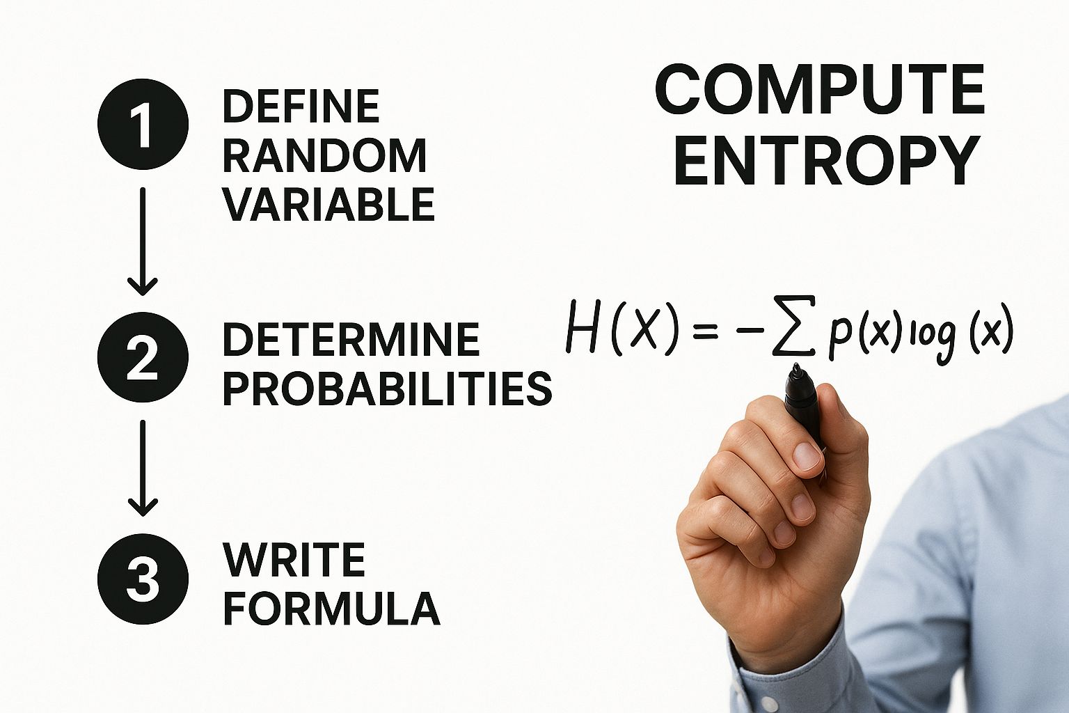
Let’s pull apart the famous Shannon entropy formula without all the dense academic speak:

H(S) = -Σ p(i) * log₂(p(i))

I know, it looks a little scary. But it's really just a few simple operations strung together. Let's walk through what each piece is doing.

Deconstructing the Entropy Formula

To really get what this equation is doing, we need to look at its three key parts:

• p(i): The Probability of Each Class
  This is the easy part. p(i) is simply the probability, or proportion, of each class i showing up in your dataset. If you have 10 data points and 7 of them are "Class A," then the probability p(A) is 7/10, or 0.7. Simple as that.

• log₂(p(i)): The 'Surprise' Factor
  Here's where the magic happens. The logarithm with base 2 (log₂) is the secret sauce. In information theory, it’s used to measure the "surprise" or the amount of information an event gives you. An event with a low probability is more surprising, so it gets a larger log value. A high-probability event is less surprising, so it gets a smaller one. Why base 2? It frames the information in terms of "bits"—think of it as the number of yes/no questions you'd need to ask to figure out the outcome.

• -Σ: The Summation
  The Greek letter sigma (Σ) is just a fancy way of saying "add it all up." The formula calculates the p(i) * log₂(p(i)) part for every single class in your dataset, and then it sums them together. That negative sign out front is there to make sure the final entropy value is always positive, because logarithms of probabilities (which are always less than 1) are negative.

In short, the formula is just a weighted average of the "surprise" for each class. It gives you a single number that represents the average amount of uncertainty across your entire dataset.

A Practical Example: Predicting Pet Adoptions

Theory is great, but let's make this real. Imagine a small dataset from an animal shelter that's trying to predict whether a dog will be adopted. Our target variable, Adopted, has two possible outcomes: 'Yes' or 'No'.

Let's say we have records for 20 dogs:

• 15 dogs found a home ('Yes').
• 5 dogs did not ('No').

Now, let's plug this into the formula, step-by-step.

1. Calculate the Probabilities (p(i))
   First up, we find the proportion of each class.

   • Probability of 'Yes' -> p(Yes) = 15 / 20 = 0.75
   • Probability of 'No' -> p(No) = 5 / 20 = 0.25

2. Calculate Each Term of the Formula
   Next, we figure out the p(i) * log₂(p(i)) value for both 'Yes' and 'No'.

   • For 'Yes': 0.75 * log₂(0.75) = 0.75 * (-0.415) = -0.311
   • For 'No': 0.25 * log₂(0.25) = 0.25 * (-2) = -0.5

3. Sum the Terms and Apply the Negative Sign
   Finally, we add these up and flip the sign.

   • H(S) = - (-0.311 + -0.5)
   • H(S) = - (-0.811)
   • H(S) = 0.811

The entropy for this dataset is 0.811. For a problem with two outcomes, the maximum possible entropy is 1 (a perfect 50/50 split). Our score of 0.811 tells us there's a moderate amount of impurity, but it's definitely more organized than a purely random mix.

Actionable Insight: Calculating Entropy with Python

Manually calculating entropy is great for understanding the concept, but for anything bigger than a toy example, you'll want to use code. Here’s just how simple it is to get the entropy for our pet adoption scenario using Python and the NumPy library.

import numpy as np

# Probabilities of our classes ('Yes' and 'No')
probabilities = np.array([0.75, 0.25])

# Calculate entropy
# Note: We filter out p=0 to avoid log(0) errors
entropy = -np.sum([p * np.log2(p) for p in probabilities if p > 0])

print(f"The entropy of the dataset is: {entropy:.3f}")
# Output: The entropy of the dataset is: 0.811

This tiny script performs the exact same calculation we just did by hand. By turning the formula into a practical tool, you can start measuring the impurity in your own datasets. This is the first and most critical step in building effective decision tree models. As we'll see in our guide on Decision Tree vs Random Forest, a solid grasp of this core mechanic is fundamental to mastering more advanced tree-based algorithms.

How Information Gain Drives Decision Trees

So now we can put a number on the "messiness" of our data using entropy. That's a great first step, but how do machine learning models actually use this number to make decisions? The answer is a simple but brilliant concept called Information Gain.

Think of Information Gain as the reward a decision tree gets for asking a good question. It’s a metric that calculates exactly how much clarity the model gains by splitting a messy dataset into cleaner, more organized subgroups. In short, it measures the reduction in entropy after partitioning the data on a specific feature.

From Chaos to Clarity: The Goal of a Split

The whole point of a decision tree is to ask a series of questions that chip away at uncertainty. It starts with a jumbled, high-entropy dataset and its goal is to create "leaf nodes" at the very end of its branches that are as pure as possible—meaning they have very low entropy.

Information Gain is the engine that drives this process. For every feature it could possibly split on, the algorithm calculates how much that split would reduce the overall entropy. The feature that delivers the biggest drop in messiness—the one with the highest Information Gain—gets chosen for that node. It's a greedy, but effective, approach.

This is a great way to visualize the process of using entropy to make these splits.

As you can see, it all starts with calculating the entropy of the dataset. This turns an abstract idea like "uncertainty" into a hard number the model can use to guide its next move.

Calculating Information Gain: A Practical Example

Let's jump back to our animal shelter example. We started with 20 dogs, where 15 were adopted ('Yes') and 5 were not ('No'). We already figured out that the entropy for this initial group (the parent node) is 0.811. That's our starting point, our baseline messiness.

Now, let's see if we can clean things up by introducing a new feature: Size ('Small' or 'Large'). We want to know if splitting the dogs based on their size will make our predictions any clearer.

Imagine our data breaks down like this:

• There are 10 Small dogs. Out of these, 9 were adopted ('Yes') and 1 was not ('No').
• There are 10 Large dogs. Out of these, 6 were adopted ('Yes') and 4 were not ('No').

The formula for Information Gain is refreshingly simple:

Information Gain = Entropy(Parent) – Weighted Average Entropy(Children)

First, we need to calculate the entropy for each of our new subgroups, or "child nodes."

1. Entropy of the 'Small' dogs subgroup:

   • Probabilities: p(Yes) = 9/10 = 0.9; p(No) = 1/10 = 0.1
   • Entropy(Small) = -[0.9 * log₂(0.9) + 0.1 * log₂(0.1)] = 0.469

2. Entropy of the 'Large' dogs subgroup:

   • Probabilities: p(Yes) = 6/10 = 0.6; p(No) = 4/10 = 0.4
   • Entropy(Large) = -[0.6 * log₂(0.6) + 0.4 * log₂(0.4)] = 0.971

You can immediately see the 'Small' group is much more predictable (lower entropy) than the 'Large' group. Now we just need to calculate the weighted average entropy of these two children.

• Weighted Avg Entropy = (Weight of Small * Entropy(Small)) + (Weight of Large * Entropy(Large))
• Weighted Avg Entropy = (10/20 * 0.469) + (10/20 * 0.971) = (0.5 * 0.469) + (0.5 * 0.971) = 0.72

Finally, we can plug this back into our original formula to get the Information Gain.

• Information Gain(Size) = 0.811 – 0.72 = 0.091

By splitting our data on the Size feature, we achieved an information gain of 0.091. The decision tree algorithm would then do this exact same calculation for every other available feature (like 'Age' or 'Breed') and pick whichever one gives the highest score. This is the core logic behind tree-based models, and you can see how it extends to more complex algorithms in our comparison of Decision Tree vs Random Forest.

Actionable Insight: Putting Information Gain into Python Code

Let's translate this logic into a quick Python function. This snippet shows you exactly how a decision tree would evaluate a potential split, connecting the theory of entropy in machine learning to a hands-on implementation you can use.

import numpy as np

def calculate_entropy(probabilities):
    """Calculates entropy given a list of probabilities."""
    # Filter out zero probabilities to avoid log(0) errors
    return -np.sum([p * np.log2(p) for p in probabilities if p > 0])

# Entropy of the parent node (15 Yes, 5 No)
entropy_parent = calculate_entropy([15/20, 5/20]) # 0.811

# Entropy of the 'Small' child node (9 Yes, 1 No)
entropy_small = calculate_entropy([9/10, 1/10]) # 0.469

# Entropy of the 'Large' child node (6 Yes, 4 No)
entropy_large = calculate_entropy([6/10, 4/10]) # 0.971

# Calculate the weighted average entropy of the children
weighted_entropy_children = (10/20 * entropy_small) + (10/20 * entropy_large) # 0.72

# Final Information Gain
info_gain = entropy_parent - weighted_entropy_children

print(f"Parent Entropy: {entropy_parent:.3f}")
print(f"Weighted Child Entropy: {weighted_entropy_children:.3f}")
print(f"Information Gain from splitting on 'Size': {info_gain:.3f}")

# Output:
# Parent Entropy: 0.811
# Weighted Child Entropy: 0.720
# Information Gain from splitting on 'Size': 0.091

Building a Decision Tree with Python

Theory is great, but let's be honest—nothing clicks until you see it in action. We've talked about how entropy and information gain are the brains behind a decision tree. Now, it's time to roll up our sleeves and translate that theory into a hands-on Python example.

We'll use Scikit-learn, the go-to machine learning library for most data scientists, along with the classic Iris dataset. This dataset is perfect for our classification task because it contains measurements for three different species of iris flowers. The goal here isn't just to run some code; it's to connect every single step back to those core ideas of entropy and information gain.

Preparing the Data for Our Model

First things first, we need to get our data in order. Luckily, the Iris dataset comes bundled with Scikit-learn, which makes getting started a breeze. We'll load the data, split it into our features (the flower measurements) and the target (the flower species), and then divide it all into training and testing sets.

The training set is what our decision tree will actually learn from. This is where all the heavy lifting happens—calculating entropy, finding the best splits using information gain, and building the tree structure. The testing set is held back, kept completely separate, so we can later see how well our model performs on data it has never seen before.

# Import necessary libraries
from sklearn.datasets import load_iris
from sklearn.model_selection import train_test_split
from sklearn.tree import DecisionTreeClassifier
from sklearn import tree
import matplotlib.pyplot as plt

# Load the Iris dataset
iris = load_iris()
X = iris.data
y = iris.target

# Split the dataset into training and testing sets
# We'll use 80% for training and 20% for testing
X_train, X_test, y_train, y_test = train_test_split(X, y, test_size=0.2, random_state=42)

print(f"Training data shape: {X_train.shape}")
print(f"Testing data shape: {X_test.shape}")

With our data prepped and ready, we can finally get to the fun part: training the model.

Training the Decision Tree Classifier

This is where the magic happens. We'll kick things off by creating an instance of DecisionTreeClassifier. There's one parameter here that's especially important for our discussion: criterion. We're going to set it to 'entropy', which explicitly tells Scikit-learn to use the information gain metric we've been learning about.

When we call the .fit() method, the algorithm springs to life:

1. It starts by calculating the initial entropy of the entire training dataset (y_train).
2. Next, it cycles through every possible split on every single feature in X_train.
3. For each one of those potential splits, it calculates the information gain—how much that split reduces the overall entropy.
4. It pinpoints the feature and threshold that delivers the highest information gain and makes that the very first split, creating the root node.
5. This entire process repeats over and over again for each new branch until the nodes are pure (entropy hits zero) or another stopping condition is met.

# Create a Decision Tree Classifier instance using entropy
# The 'random_state' ensures our results are reproducible
clf = DecisionTreeClassifier(criterion='entropy', random_state=42)

# Train the model on our training data
clf.fit(X_train, y_train)

print("Decision Tree model trained successfully!")

Actionable Insight: It's pretty amazing what's going on under the hood. In just a couple of lines, Scikit-learn is running thousands of entropy and information gain calculations. This powerful abstraction lets us focus on the bigger picture and interpret the model's logic, rather than getting stuck in the weeds of manual math.

Of course, after a model is trained, it's critical to track its performance over time. Data can drift, and accuracy can suffer, so having a solid plan for machine learning model monitoring is essential for keeping your model reliable in a production environment.

Visualizing the Decision-Making Process

One of the biggest wins for decision trees is how easy they are to interpret. We don't have to treat our model like an unexplainable black box. Instead, we can actually visualize the exact rules it learned from the data. Plotting the tree lets us trace the journey from the root node all the way down to a final prediction, giving us a clear view of how entropy guided the creation of every split.

The code below will generate a picture of our tree, showing the splitting rules, the entropy at each node, and how many samples fall into each bucket.

# Set up the figure size for better readability
plt.figure(figsize=(20,10))

# Visualize the tree
tree.plot_tree(clf,
               feature_names=iris.feature_names,
               class_names=iris.target_names,
               filled=True)

plt.title("Decision Tree for Iris Classification (Criterion='entropy')")
plt.show()

Take a look at the resulting image. You can see the initial entropy at the root node and watch how each split creates child nodes with lower and lower entropy. This visualization is the perfect confirmation of how the algorithm systematically works to reduce uncertainty, step by step, building a clear and logical flowchart for classifying iris flowers. It's a fantastic way to solidify the link between the abstract concept of entropy in machine learning and its very real, practical application.

Entropy Beyond Decision Trees in Modern ML

While decision trees are the classic playground for understanding entropy, its real influence stretches far beyond those simple branching structures. The core ideas of measuring uncertainty and information are fundamental to a massive range of modern machine learning algorithms, acting as a guiding principle for building and tuning even the most complex systems.

One of its most important descendants is cross-entropy, a variation that has become the go-to loss function for pretty much any modern classification model. Think of it as a way to measure the "distance" between your model's predicted probabilities and the actual truth on the ground.

For instance, if your model is 90% sure an image is a cat, but it's really a dog, cross-entropy is what quantifies that mistake. A lower cross-entropy score means your model's predictions are getting closer and closer to reality. This simple but powerful idea is what makes it indispensable for training everything from basic logistic regression models to the massive deep neural networks powering today's AI.

Guiding Advanced Algorithms

The principles of entropy also shape how more advanced models learn and explore their solution space. Its role has ballooned since the 1980s, finding its way into probabilistic and energy-based models. Concepts borrowed directly from statistical mechanics and entropy, for example, are central to how energy-based models like Boltzmann machines optimize their internal states. It's a fascinating connection, showing how a concept from physics has become a powerful tool for dissecting complex datasets. For a deeper dive, you can read more about how entropy is used to measure data structure and redundancy in this detailed study on its applications.

Entropy's reach can be spotted in several other key areas:

• Reinforcement Learning (RL): In RL, an agent learns through trial and error. Entropy is often tossed into the agent's objective function as an "entropy bonus." This clever trick encourages the agent to explore a wider variety of actions instead of just getting stuck on the first strategy that works. It stops the model from becoming too predictable and helps it stumble upon more creative and robust solutions.
• Clustering Quality: In the world of unsupervised learning, entropy can be a great report card for how well your clustering algorithm performed. After an algorithm like K-Means has grouped your data, you can measure the entropy within each cluster. A low-entropy cluster is pure and well-defined, full of similar items—a clear signal the algorithm did a great job.
• Feature Engineering: Understanding the entropy of your features can be a huge help in feature engineering for machine learning. A feature with super low entropy (meaning almost all its values are the same) isn't providing much information and is probably a good candidate to be dropped.

A Practical Example in Natural Language Processing

Let's look at building a language model. The model's job is to predict the next word in a sentence.

If you give it the sentence, "The cat sat on the…", the next word is almost certainly "mat." The probability distribution for what comes next has very low entropy because there’s not much uncertainty. But for a sentence like "Her favorite activity is…", the possibilities are endless—"reading," "hiking," "coding," you name it. That distribution has high entropy.

Models like GPT use cross-entropy during training to measure how "surprised" they are by the correct next word. Minimizing this surprise across trillions of examples is precisely what makes them so uncannily good at generating text. As we tackle more sophisticated jobs, like training machine learning models for chatbots, these fundamental principles of entropy are always there, working behind the scenes to optimize performance.

This just goes to show that entropy in machine learning isn't some dusty, historical footnote tied to decision trees. It’s a living, breathing principle that helps us quantify uncertainty, guide exploration, and squeeze every last drop of performance out of the most powerful models we use today.

Actionable Tips for Your Machine Learning Projects

Understanding the theory behind entropy in machine learning is one thing, but applying it effectively is what separates good models from great ones. Moving from concept to practice really comes down to making strategic choices that can seriously boost your model's performance and interpretability.

The most common application you'll run into is feature selection in tree-based models. By calculating the information gain for each feature, you can literally rank them by their power to reduce uncertainty. Features with high information gain are your most valuable predictors, while those with little to no gain might just be adding noise. This entropy-driven approach helps you build simpler, more robust models that are far easier to explain.

Choosing Between Entropy and Gini Impurity

When you're building a decision tree, you'll often face a choice between criterion='entropy' and criterion='gini'. They often produce very similar results, but there are some subtle differences worth knowing.

• Entropy: Tends to create more balanced trees. The logarithmic calculation is slightly more computationally intensive, which can be a factor on very large datasets.
• Gini Impurity: Is faster to compute and is often the default in libraries like Scikit-learn for a reason. It has a tendency to isolate the most frequent class in its own branch.

Actionable Insight: Start with the default (Gini) for speed, but don't hesitate to experiment with entropy, especially if your classes are imbalanced or if interpretability is a high priority. Sometimes, the slightly different splits that entropy produces can uncover valuable patterns that Gini misses.

Managing High-Cardinality Features

Features with tons of unique values—think user IDs or zip codes—can be a real trap. They often appear to have high information gain simply because they can split the data into many pure, tiny nodes. The problem? This rarely generalizes to new, unseen data and is a classic sign of overfitting.

Actionable Insight: Use entropy-based metrics as a guide, not a blind rule. When a high-cardinality feature rockets to the top of your information gain list, be skeptical. Consider feature engineering techniques like grouping categories or using target encoding to make the feature more meaningful first.

Entropy in Anomaly Detection and Data Compression

Beyond decision trees, entropy has some other powerful applications. For instance, in anomaly detection, unusual data points often disrupt the expected "order" or low-entropy state of a system. A sudden spike in the entropy of a data stream can be a powerful signal of a potential outlier or system failure.

Entropy also plays a huge role in information compression and cryptography. Shannon's information entropy defines the absolute minimum number of bits needed to encode data without loss, which is the foundation for standards like JPEG and MP3. This same principle helps machine learning systems optimize data storage. For example, statistical analysis shows that entropy-based compression can improve ratios by 10-30% on diverse datasets compared to naive methods, saving vast amounts of storage globally.

Developers looking to integrate AI into their projects can benefit from exploring these highly-rated tools. Check out this list of the Top AI Tools for Developers to find resources that can streamline your workflow.

Common Questions About Entropy

When you're first getting your head around entropy in machine learning, a few questions always seem to pop up. Let's tackle them head-on.

What's the Difference Between Entropy and Gini Impurity?

Think of them as two different tools for the same job. Both Entropy and Gini Impurity are used in decision trees to figure out how "mixed up" a node is, and honestly, they usually give you very similar results.

The key difference is in their sensitivity. Entropy’s logarithmic function makes it a bit more responsive to small changes in class probabilities, which can sometimes lead to more balanced trees. Gini Impurity, on the other hand, is quicker to calculate and has a knack for isolating the most dominant class in its own branch, which can be a useful trait.

Why Use Log Base 2 in the Entropy Formula?

That log₂ isn't just for show—it's a direct nod to information theory, where Claude Shannon first framed information in terms of "bits."

A bit is the smallest possible unit of information, essentially a single "yes" or "no" answer. By using log base 2, we can interpret the entropy value in a really intuitive way: it's the average number of yes/no questions you'd need to ask to correctly guess the class of any given sample.

How Do You Handle Continuous Variables?

This is a great question. Decision trees are built on splits, but how do you split something that isn't a neat category, like age or temperature?

The algorithm handles this by finding the best possible split point. It starts by sorting all the continuous values in a feature. Then, it tests every possible threshold to see which one creates the purest nodes—in other words, which split gives the highest information gain. For instance, it might check thousands of values for "age" and discover that splitting the data at > 35 years old is the single most effective way to reduce entropy.

---

At DATA-NIZANT, our goal is to make complex data science concepts clear and actionable. Knowing how to apply these ideas is what drives real business value, a topic we explore further in our guide to leveraging AI in business.