Why Covariance Matrices Matter More Than You Think

Covariance matrices are essential in data analysis. They’re like a map, revealing the hidden connections within your data. Imagine you’re trying to figure out how website traffic, social media buzz, and actual sales connect. A covariance matrix helps you see these relationships, showing which factors move together and which go their own way.

This interconnectedness is where the real power lies. Let’s say you’re looking at a stock portfolio. A covariance matrix can show you how the different stocks relate to one another. This is key for managing risk. If all your stocks tend to move in the same direction, a market dip could really hurt. A covariance matrix calculator like those you can find online helps you see these patterns so you can build a safer, more diverse portfolio.

Speaking of finance, the RiskMetrics model, developed by J.P. Morgan in 1994, really brought covariance matrices to the forefront of risk management. Think about managing a global portfolio with stocks from 20 different markets. The covariance matrix shows how the returns of these stocks vary together. This became a gold standard, influencing how financial institutions everywhere assess and manage risk. Want to dive deeper into financial risk? Learn more about financial risk assessment.

Covariance matrices aren’t just for finance, though. They pop up everywhere! From machine learning algorithms to image processing and even social science research, they’re a valuable tool. Anytime you have multiple variables at play, a covariance matrix can shed light on how they interact. Speaking of valuable tools, check out this guide on statistical significance and confidence intervals. Mastering covariance matrices can seriously level up your data analysis game.

Calculating Covariance Matrices That Actually Make Sense

Covariance matrices. They sound complicated, right? Like something you’d need a PhD in statistics to understand. Honestly, they’re not that bad. Think of them as a way to see how different parts of your data relate to each other – a snapshot of their interactions. Imagine you’re trying to figure out what affects sales at your coffee shops. You’re looking at the temperature, the humidity, and the price of a latte. The covariance matrix would show you how these factors play together. Does high humidity mean fewer iced coffees sold? Does the temperature affect how much people are willing to pay for a hot drink? That’s the kind of insight a covariance matrix can unlock.

Let’s dive into how to actually calculate these matrices and, more importantly, how to make sense of them.

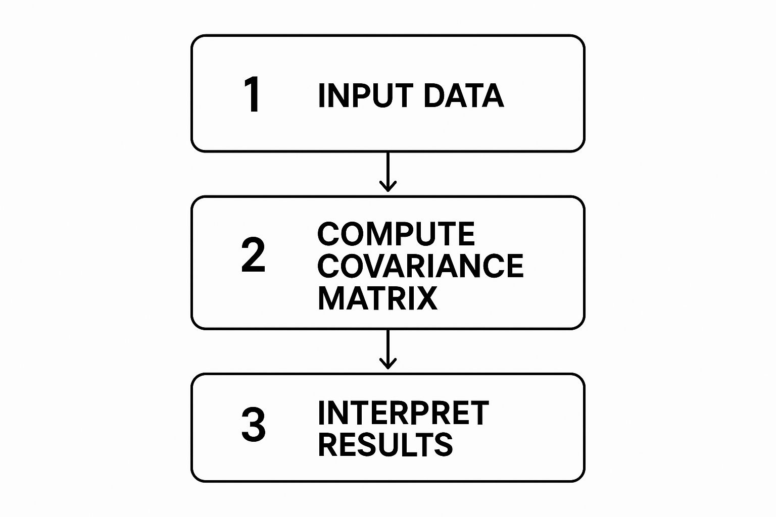
This infographic shows the whole process of using a covariance matrix calculator: input the data, calculate the matrix, and then interpret what it all means. It’s a straightforward three-step flow. We’re going from raw data to a real understanding of the relationships hiding within.

Population vs. Sample: Choosing the Right Approach

Now, there are two main ways to calculate a covariance matrix: the population method and the sample method. The population method is what you use when you have data on everything you’re interested in. For example, if you’re analyzing test scores for every single student in a class, that’s your population. You’d use the population method. The sample method, on the other hand, is for when you only have a piece of the puzzle – a sample of the data. Like if you’re looking at a random selection of customer reviews instead of every single one.

Picking the right method really depends on what you’re working with and what you’re trying to find out. In my experience, the sample method is usually more realistic, especially with huge datasets. Getting data on an entire population is often just not possible.

Breaking Down the Math

The basic idea behind covariance is to measure how much two variables move together, away from their average values. A positive covariance means they generally move in the same direction. A negative covariance means they tend to move in opposite directions. Imagine you’re tracking website traffic and how much you’re spending on ads. A positive covariance would suggest that as your ad spend goes up, so does your website traffic.

Speaking of analyzing trends, you might find time series analysis helpful. If you’re using Python, our guide on ARIMA in Python might be useful for digging deeper into those techniques.

When you’re calculating a covariance matrix, you’re doing this calculation for every possible pairing of variables in your data. The results get arranged in a matrix. The diagonal of the matrix shows the variance of each variable (how much it varies on its own). The matrix is always symmetrical. This means the covariance between Variable A and Variable B is the same as between Variable B and Variable A. Each number in the matrix tells a story about the relationship between two variables. By understanding those individual stories, we can start to understand the bigger picture the covariance matrix paints.

Let’s look at how the population and sample approaches differ in practice.

To help illustrate the differences, here’s a table summarizing each method:

Population vs Sample Covariance Methods

Method	Formula	When to Use	Advantages	Limitations
Population	σ_xy = (1/N) * Σ[(x_i – μ_x)(y_i – μ_y)]	When you have data for the entire population	Accurate for the population being studied.	Difficult or impossible to obtain data for the entire population in many real-world scenarios.
Sample	s_xy = (1/(n-1)) * Σ[(x_i – x̄)(y_i – ȳ)]	When you have data for a sample of the population	More practical for large datasets or when complete population data is unavailable. Provides an unbiased estimate of the population covariance.	Less accurate than the population method if the sample is not representative of the population.

This table highlights when you’d choose each method, their strengths, and what to watch out for. Notice the difference in the denominators (N vs. n-1). This seemingly small difference is key to ensuring the sample covariance is an unbiased estimator of the population covariance.

As you can see, both methods offer valuable insights, but picking the right one depends on your specific situation and the data you have available.

Solving Problems When Calculations Go Wrong

Let’s be honest, real-world data is rarely as pristine as the examples you see in textbooks. Forget those perfectly organized datasets; in practice, you’re more likely to encounter missing values, formatting inconsistencies, and situations where you have way more variables than observations. These aren’t just theoretical problems; they’re the daily struggles that can make covariance matrix calculations a real pain.

Imagine working with survey data where a significant portion of respondents skipped a key question. Standard covariance formulas can’t handle those missing data points, potentially derailing your entire analysis.

Handling High-Dimensional Data

Another common issue is having more variables than observations. Think about genetic studies, where you might be tracking thousands of genes but only have data from a few hundred participants. This can lead to singular matrices, which are essentially matrices that can’t be inverted. This is a big deal because many statistical techniques, especially those used with covariance matrix calculators, depend on matrix inversion. Without it, your analysis comes to a screeching halt.

Covariance matrices are fundamental in statistical analysis, especially when dealing with multivariate data. When the number of variables is greater than the number of observations, traditional covariance estimation methods can produce these problematic singular matrices. Shrinkage estimation techniques, like the Ledoit-Wolf method, offer a solution. They blend the empirical estimator with a target matrix to create a more stable and reliable estimate. This is particularly helpful in methods like Principal Component Analysis (PCA) and factor analysis, where accurate covariance matrices are crucial for extracting meaningful information. For a deeper dive into covariance matrices and estimation methods, check out this resource: Estimation of Covariance Matrices.

So, how do you fix these problems? Unfortunately, there’s no single easy answer. It’s more about having a range of strategies at your disposal. For missing data, imputation techniques can fill in the gaps using smart estimates based on the available data. For high-dimensional data, techniques like regularization or the shrinkage estimation mentioned earlier can help stabilize your covariance matrix and avoid those troublesome singular matrices.

The important thing to remember is that calculating covariance matrices isn’t simply about plugging numbers into a formula. It’s about understanding the potential issues and having the know-how to address them. By anticipating these challenges, you’ll be much better prepared to generate covariance matrices that are both meaningful and provide reliable insights.

Programming Your Way Through Covariance Calculations

Ready to ditch the pencil and paper and let your computer handle those covariance calculations? Let’s dive into how to calculate covariance matrices using Python and R, the tools data scientists rely on daily. From my experience, understanding both is a huge asset, as they each have their own strengths.

Python: NumPy and Pandas For the Win

In the Python world, NumPy and Pandas are your best friends for covariance calculations. NumPy provides the core mathematical muscle, while Pandas offers incredibly useful data structures and functions specifically designed for real-world data – especially those messy CSV files we all know and love (or maybe not so much).

Imagine you’re working with stock price data from a CSV file. Pandas makes importing and cleaning that data straightforward. You can easily deal with missing values (those pesky blank cells) and make sure your data types are correct, prepping everything perfectly for analysis. Then, the .cov() function in Pandas calculates the entire covariance matrix in one go.

Here’s a quick example:

import pandas as pd

Load your data

data = pd.read_csv(“stock_prices.csv”)

Calculate the covariance matrix

covariance_matrix = data.cov()

print(covariance_matrix)

This code snippet shows how easy Pandas is to use. It handles all the behind-the-scenes complexity so you can focus on the results. Keep in mind, .cov() defaults to calculating the sample covariance matrix. If you need the population covariance, NumPy’s np.cov() function lets you specify a bias correction.

R: Built-In Power for Statistical Analysis

R, built specifically for statistical computing, has covariance calculations built right in. The cov() function is your key tool here. Like Pandas, it smoothly handles various data structures, and you can choose between population or sample covariance.

Assuming ‘my_data’ holds your data

covariance_matrix <- cov(my_data)

print(covariance_matrix)

R’s real power is in its comprehensive statistical environment. After calculating the covariance matrix, you can seamlessly integrate it into other analyses, like principal component analysis or linear regression, all within the same system. I’ve personally found this incredibly efficient for streamlining involved workflows.

Handling Real-World Messiness

Textbooks rarely prepare you for the real-world challenges of data cleaning and formatting. Suppose your dataset has dates stored as text. Both Python and R have the tools to convert these into the right format for calculations. Or maybe you have inconsistent units across your variables. Tackling these practical hurdles before calculating your covariance matrix is essential for accurate and meaningful results. This pre-processing stage is where experience really pays off. Knowing the quirks of your data and which tools to use will save you hours of frustration.

Let’s talk tools! To help you choose the right tool for your covariance analysis, I’ve put together this comparison table:

To help you choose the right environment for your analysis, I’ve put together this handy table:

Programming Tools for Covariance Analysis
Practical comparison of languages and tools for covariance matrix calculations, including ease of use and capabilities.

Tool	Key Functions	Main Libraries	Learning Curve	Best Applications
Python	.cov(), np.cov()	NumPy, Pandas	Moderate	Data cleaning, general-purpose analysis, scripting
R	cov()	Base R	Moderate	Statistical modeling, in-depth analysis

This table highlights the strengths of each tool. Python, with its Pandas library, excels at data manipulation and cleaning. R, on the other hand, shines in statistical analysis.

Calculating the covariance matrix is just the first step. The real value comes from understanding what those numbers mean. This is where visualization tools and other analytical techniques become invaluable. We’ll explore these in more detail later.

Online Calculators That Actually Work

Let’s be honest, sometimes you just need a covariance matrix quickly. Crunching those numbers by hand takes time, especially with a massive dataset. That’s when a solid online covariance matrix calculator becomes your best friend. But finding one that’s reliable and user-friendly? That can be tricky.

I’ve spent my fair share of time battling with these tools, so let me share some tips on getting quick, accurate results. One common trap is incorrect data input. Many calculators expect data in a very specific format (often comma-separated values), and even tiny errors or inconsistencies can mess things up. Double-checking the data formatting before hitting “calculate” is a lifesaver. Trust me. Speaking of reliable online calculators, take a look at this one from SolveMyMath. It’s a great way to quickly calculate covariance matrices, especially for multivariate data when you need a covariance estimate without needing a PhD in statistics.

For example, imagine you’re analyzing stock prices. You can use this calculator to pinpoint correlations quickly, which can be incredibly helpful for making smart investment decisions.

This screenshot shows the SolveMyMath covariance calculator in action. The input format is simple – just enter your data. The matrix is calculated instantly. The output is clear and concise, displaying the computed covariance matrix. It’s also easy to copy and paste the results into other applications.

Choosing the Right Calculator for the Job

Another important factor is dataset size. Some online calculators handle large datasets smoothly, while others choke. I’ve noticed some tools limit the number of variables or observations you can input, so it’s a good idea to check those limits beforehand.

Some calculators also offer extra features like visualization. Seeing the covariance matrix visually can help you spot patterns and understand the relationships between variables. It’s usually much easier than staring at rows and columns of numbers.

Verifying Your Results

Finally, always double-check your results. Does the output make sense given your data? If anything looks strange, there’s probably an issue with the input or calculation. I find it helpful to compare the online results with a quick manual calculation using a small chunk of the data or cross-check with software like Python or R. This helps build confidence in the results and catches errors early. Knowing when to rely on an online calculator and when to switch to more robust software is a skill that comes with practice. These tools are fantastic for quick analyses, but more complex scenarios might require dedicated statistical packages.

Turning Numbers Into Insights That Matter

So, you’ve got your covariance matrix, maybe from a handy covariance matrix calculator, and you’re looking at a grid of numbers. What now? Honestly, this is where the real work begins. It’s tempting to just stare blankly, but the power lies in understanding what those numbers mean. Let’s unpack how to turn that matrix into useful insights.

Deciphering the Covariance Code

Every number in your covariance matrix tells a story about the relationship between two variables. A positive covariance means they tend to move together. Imagine website traffic and leads – more traffic, more leads (hopefully!). That’s a positive covariance in action. A negative covariance, on the other hand, indicates an inverse relationship. Think product price and demand. Price goes up, demand often goes down. And if a covariance is close to zero? The variables are likely independent – what happens to one doesn’t really affect the other.

In my experience, though, the actual size of the covariance isn’t super helpful on its own. That’s where correlation comes in. Correlation standardizes covariance to a manageable scale between -1 and 1. This makes comparing relationships much easier. A correlation close to 1 or -1 signifies a strong relationship, while something around 0 means a weak relationship.

Beyond Correlation: Causation vs. Connection

Here’s a crucial point: correlation isn’t causation. Just because two variables move in sync doesn’t mean one causes the other. Let me give you an example. Two stocks might show a strong positive correlation, but that doesn’t mean one’s performance directly influences the other. Other market factors could be driving both.

Spotting Troublemakers: Outliers and Skewed Results

Outliers, those weird data points far from the rest, can really mess with your covariance matrix. Just one extreme value can inflate your covariances, leading to inaccurate conclusions. I always recommend visualizing your data first. A simple scatterplot can reveal outliers, giving you a chance to investigate and decide whether to remove, adjust, or further analyze them. This often leads to a much cleaner picture of the real relationships.

Communicating Your Findings

Let’s talk about sharing your insights. A raw covariance matrix is about as exciting as watching paint dry. Visualizations like heatmaps, on the other hand, can be incredibly powerful. They visually represent the strength and direction of the covariances, making complex relationships immediately obvious. And remember, clear explanations are key! Translate those statistical findings into plain language, emphasizing the practical takeaways and what actions to consider.

Your Complete Covariance Matrix Toolkit

So, you’ve crunched covariance matrices every which way – by hand, with Python and R, and even using online calculators. Think of this section as your cheat sheet, a quick pit stop to refresh your memory and troubleshoot any covariance curveballs.

Essential Formulas and Common Pitfalls

Let’s start with the essentials. Keep these formulas handy:

• Population Covariance: σ_xy = (1/N) * Σ[(x_i – μ_x)(y_i – μ_y)]
• Sample Covariance: s_xy = (1/(n-1)) * Σ[(x_i – x̄)(y_i – ȳ)]

Even after years of working with these, I’ve still seen some common slip-ups. Here’s what to watch out for:

• Data Mismatches: Seriously, double-check your data. Make sure your dates, units, and everything else lines up perfectly. Even a small mismatch can wreck your results.
• Outlier Neglect: Outliers are those sneaky data points that can seriously skew your covariance. Visualize your data first to spot and handle them. A simple scatter plot can be a lifesaver here.
• Correlation vs. Causation Confusion: Just because two variables move together doesn’t mean one causes the other. Covariance measures how they change together, not why.

Troubleshooting Tricky Situations

Sometimes, things just don’t go as planned. Here are a couple of common headaches and how to fix them:

• Missing Data: Don’t panic! Imputation techniques can help. These methods use the existing data to make educated guesses about those missing values.
• High-Dimensional Data (More Variables Than Observations): This can make your covariance matrix go wonky. Regularization and shrinkage estimation can help stabilize things and prevent it from becoming singular (non-invertible).

Software Recommendations and Practical Tips

For your day-to-day covariance calculations, Python with Pandas and NumPy is usually a great choice. R is fantastic when you need to do some serious statistical modeling. By the way, you might find our guide on Python for topic modeling useful. Online covariance matrix calculators are handy for quick answers, but be careful with large datasets – they might have limitations.

My advice? Start small. Practice with small datasets to build your intuition. Don’t be afraid to play around and try different things. Focus on understanding why you’re doing each calculation. That’s how you build confidence in your analysis and learn to communicate your findings effectively.

Ready for more data science adventures? Check out DATA-NIZANT for a treasure trove of resources on data, AI, and machine learning.