Why LSTM Networks Excel at Time Series Prediction

After building countless forecasting models, I’ve developed a real appreciation for LSTM networks. For complex time series, they just consistently outperform traditional methods. Think about it: traditional approaches often treat each data point like it’s on its own little island, completely ignoring the connections and dependencies within the sequence. That’s where LSTMs shine.

LSTMs have these things called memory cells. Imagine them as your own personal time-traveling assistant, remembering key events that influence future predictions. This “memory” allows them to filter out the noise and focus on the important stuff – the underlying trends and patterns. It’s like having a data detective on your team.

How LSTM Memory Works

This memory magic happens thanks to three clever gate mechanisms: the forget gate, the input gate, and the output gate. The forget gate is like a decluttering guru, tossing out old information that’s no longer relevant. The input gate is the selective librarian, carefully choosing which new data is worth keeping. And finally, the output gate is the spokesperson, deciding what information from memory is shared to make the next prediction.

You can visualize this whole process with the diagram on the Wikipedia page for Long Short-Term Memory. It shows how information flows through the memory cell and how the gates control everything. Really understanding this flow helps you appreciate the power of LSTMs. It’s not just about feeding data in – it’s about the network’s ability to learn and remember sequential patterns.

Real-World Examples

Let’s say you’re forecasting retail demand. LSTMs can handle things like seasonal shopping spikes, long-term growth trends, and even the impact of a flash sale or a supply chain hiccup. Or, imagine predicting energy consumption. LSTMs can take into account daily and weekly usage patterns, and even factor in weather changes. These are the subtle details that simpler models, like ARIMA, often miss.

One of the biggest reasons LSTMs are so effective with sequential data is their ability to sidestep the vanishing gradient problem that plagues traditional neural networks. This means they can maintain context even over long sequences, which is hugely beneficial for things like long-term weather forecasting or resource planning.

Choosing the Right Tool

Now, a word of caution. While LSTMs are powerful, they’re not a one-size-fits-all solution. If you’re dealing with a simple time series with obvious linear patterns, a traditional method might be faster and less likely to overfit. The trick is knowing which tool is best for each specific job – sometimes a simple wrench is better than a high-powered drill.

Transforming Raw Data Into LSTM-Ready Format

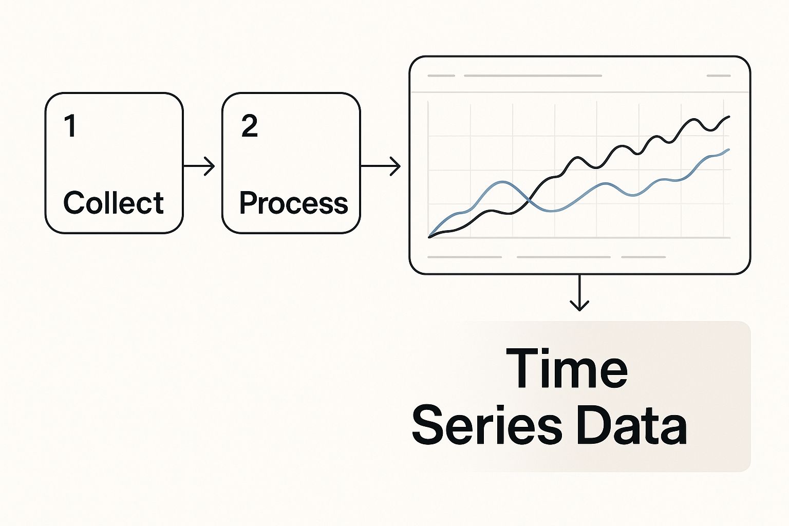
The infographic above gives you a visual taste of time series data. See how the lines dance and intertwine? That’s the sequential nature of the data, a key element for LSTMs. Preparing your data is all about making these relationships crystal clear for the network.

Now, let me tell you, prepping time series data for LSTM forecasting isn’t as easy as it sounds. It’s not a simple matter of plugging in the data and hitting “go.” It’s more like detective work, requiring you to understand the data’s unique characteristics, hidden patterns, and potential problems. I’ve spent countless hours debugging models, only to discover a tiny preprocessing error was the root of all evil. Trust me, this stage is where LSTM projects either take off or crash and burn.

Exploring and Cleaning Your Data

First things first: data exploration. What’s the data’s frequency? Daily, hourly, something else? Are there gaps in the data? Any oddball values sticking out like sore thumbs? Missing values can mess up your LSTM training like a flat tire on a race car, while outliers can lead your model down the wrong path, causing it to learn the wrong lessons. I once worked on a sensor data project where a few faulty readings, which initially seemed trivial, totally skewed the model’s predictions. A simple outlier detection technique, like the Interquartile Range (IQR) method, could have saved weeks of headaches.

So, fixing these issues is mission-critical. You might fill in missing values with methods like linear interpolation or fancier techniques like K-Nearest Neighbors (Scikit-learn). For outliers, you might trim them down to size or use robust scaling. The best approach depends on the quirks of your dataset and the problem you’re tackling.

The Magic of Supervised Learning

Here’s where the real magic happens: turning your sequential data into a supervised learning problem. This involves crafting input-output pairs that teach the LSTM network how past patterns connect to future values. Imagine showing the LSTM flashcards: “Here’s a sequence of past stock prices. What do you think the price will be tomorrow?”

This transformation often involves a sliding window technique. Choosing the right window size—the number of past time steps fed as input—is key. A small window might miss long-term trends, while a large one might make the model too slow to react to recent changes. Finding that sweet spot is often more art than science, requiring careful experimentation.

Scaling and Feature Engineering

Preprocessing is the unsung hero of time series forecasting with LSTMs. This involves framing the time series as a supervised learning task, making sure the data is stationary, and scaling things appropriately. You can judge the effectiveness of this with metrics like Mean Absolute Error (MAE) or Root Mean Squared Error (RMSE). Want to dive deeper? Discover more insights.

Scaling your data is another big factor for LSTM performance. MinMax scaling, compressing data between 0 and 1, is common. But standardization (z-score normalization) might be better if your data looks like a bell curve or has outliers. I once saw a 10% accuracy boost just by switching from MinMax to standardization!

Finally, don’t forget feature engineering! While everyone loves tweaking network architectures, sometimes the biggest wins come from simple features like lagged values, rolling averages, or even pulling in data from external sources. In one project forecasting energy consumption, adding weather data as a feature supercharged our model’s accuracy.

Let’s talk about data preprocessing techniques for a moment. The table below summarizes some common methods, their use cases, pros, cons, and when they are most effective. This gives you a handy quick reference for making informed decisions about your data preparation strategy.

Technique	Use Case	Advantages	Disadvantages	When to Use
MinMax Scaling	Normalizing data to a specific range (0-1)	Simple to implement, preserves data distribution shape	Sensitive to outliers	When data doesn’t follow a Gaussian distribution and outliers aren’t a major concern
Standardization (Z-score normalization)	Transforming data to have zero mean and unit variance	Handles outliers well, improves model convergence	Doesn’t bound the data to a specific range	When data is approximately Gaussian or when outliers are present
Log Transformation	Reducing the impact of large values	Helps stabilize variance, improves model performance on skewed data	Can’t be applied to negative or zero values	When data is positively skewed
One-Hot Encoding	Converting categorical variables into numerical representations	Suitable for nominal data, avoids creating artificial ordinal relationships	Increases the number of features	When dealing with categorical variables that don’t have an inherent order
Label Encoding	Assigning numerical labels to categorical values	Simple, doesn’t increase feature dimensionality	Can introduce artificial ordinal relationships	When dealing with ordinal categorical variables

As you can see, each technique has its strengths and weaknesses. Choosing the right one, or even combining several, is a crucial step in getting your data LSTM-ready.

Architecting LSTM Models That Actually Perform

Building a good LSTM network for time series forecasting isn’t about blindly adding layers. It’s more like picking the right tool from a toolbox. Sometimes, a simple, well-tuned single-layer LSTM is far better than a complex, multi-layer monster. From my experience, over-engineering often leads to more headaches than improved results.

Finding the Sweet Spot for LSTM Units

LSTM units are the core building blocks of your network. The number you choose directly affects how much the model can learn. Too few, and it’s like trying to paint a masterpiece with a single, tiny brush. Too many, and you’re likely to overfit – like memorizing the training data instead of actually learning the underlying patterns. A good starting point is 32 or 64 units. Then, gradually increase this number until performance plateaus on your validation set. This sweet spot prevents overfitting and optimizes your model’s performance.

Dropout: Preventing Overfitting Without Killing Learning

Overfitting is a common LSTM problem. Dropout helps prevent this by randomly ignoring a percentage of neurons during training. Think of it as forcing your network to learn multiple ways to solve the problem, preventing it from relying too heavily on any single neuron. I often find a dropout rate between 0.2 and 0.5 works best. In one project, a dropout rate of just 0.3 significantly reduced overfitting without hindering the model’s learning ability.

Batch Size: Balancing Efficiency and Stability

Batch size – the number of samples processed before updating the model – affects both training speed and gradient stability. Larger batches are like taking giant steps – faster, but potentially less stable. Smaller batches are like taking smaller, more precise steps – slower but more accurate. A good range to experiment with is between 16 and 128. I often begin with 32 and then tweak it depending on the dataset’s size and the available computational power.

Bidirectional LSTMs: When Two Directions Are Better Than One

Bidirectional LSTMs process data in both forward and reverse directions. This can be useful when future context is important, like in natural language processing. However, for time series forecasting, often only the past is relevant. In these cases, a standard LSTM might be sufficient. If you’re looking at other time series methods, you might find our guide on mastering ARIMA in Python helpful.

Encoder-Decoder Architectures: Elegant Multi-Step Forecasting

Encoder-decoder architectures are a slick way to handle multi-step predictions. Imagine summarizing a long story into a short, concise message – that’s the encoder. Then, the decoder takes this message and expands it back into a detailed narrative, this time, the future of your time series. I’ve used this for predicting multiple future steps with excellent results.

From Theory to Practice: Avoiding Costly Mistakes

Lots of LSTM architectures look great on paper but don’t perform well in real-world situations. Some are computationally expensive, while others are overly sensitive to hyperparameter changes. I’ve learned that the simplest architecture that gets the job done is often the best. It’s all about finding the right balance between complexity and practicality. Thorough testing and evaluation on a held-out test set are vital for avoiding expensive mistakes down the line.

Training Approaches That Deliver Consistent Results

Training LSTM networks for time series forecasting isn’t quite like training other machine learning models. It’s not a set-it-and-forget-it situation. The sequential nature of the data demands a different approach, and it all begins with how you split your data for training and testing. Trust me, splitting time series data like you would with tabular data is a huge mistake. You’ll get fantastic results in testing, only to see them fall apart in the real world. Your validation set must come after your training set chronologically. Otherwise, it’s like giving your model a glimpse into the future – not exactly fair, is it?

Learning Rate Strategies: Finding the Sweet Spot

Picking the right learning rate is crucial. Think of it like finding the right speed for a road trip. Too slow, and you’ll never get there. Too fast, and you risk a crash. One common problem is getting stuck in local minima, those pesky little dips in the loss landscape. It’s like your car getting stuck in a pothole. Adaptive learning rate methods, like Adam and RMSprop, are a game-changer here. They dynamically adjust the learning rate during training, helping you navigate those tricky spots more effectively. They’re like a smart cruise control system for your model.

Early Stopping: Preventing Overfitting

Overfitting is a constant worry with LSTMs. It’s like a student memorizing the textbook instead of understanding the material. Early stopping is your solution. It keeps a close eye on the model’s performance on a validation set and stops the training process as soon as performance starts to decline. This prevents the model from getting too specialized to the training data. It’s like a teacher stepping in when a student starts reciting answers without genuine understanding.

Batch Training Approaches: Balancing Speed and Stability

Batch training involves feeding the model data in chunks. Larger batches are like taking bigger steps – potentially faster, but requiring more resources. Smaller batches are like shorter, more careful steps – more stable, but possibly slower. The ideal batch size depends on your hardware and dataset. I usually start with 32 and experiment from there. In one project, bumping the batch size up to 64 significantly cut training time without sacrificing performance.

Understanding LSTM Loss Curves and Gradients

LSTM loss curves can be a bit wild, especially early on. They can fluctuate quite a bit, making it harder to tell if your model is actually converging. It’s like watching a race where the runners stumble at the start before finding their stride. You also need to watch out for vanishing and exploding gradients. These issues can completely derail the learning process. Keeping an eye on gradient norms during training can help you catch these problems.

Practical Monitoring and Patience is Key

Training LSTMs requires patience. It’s a marathon, not a sprint. Regular monitoring of key metrics like loss, validation performance, and gradient norms is essential. Tools like TensorBoard (TensorBoard) are invaluable for visualizing these metrics and spotting potential issues. I’ve had projects where training took hours, even on powerful hardware. Seeing the slow, steady progress on TensorBoard kept me from giving up too early. Remember, reaching a stable performance plateau often takes longer than you might initially expect.

Introducing the LSTM Training Parameters Guide, a handy table summarizing essential training parameters, their typical ranges, the impact they have on model performance, and recommended starting values for various time series data types. Remember, these are guidelines, not strict rules – a starting point for your own experimentation.

Parameter	Typical Range	Impact	Recommended Start	Tuning Tips
Learning Rate	1e-5 to 1e-2	Controls the step size during training	1e-3	Use adaptive learning rate methods like Adam
Batch Size	16 to 256	Affects training speed and gradient stability	32	Experiment with different sizes
Epochs	50 to 500	Number of training iterations	100	Monitor validation loss for early stopping
Dropout Rate	0 to 0.5	Prevents overfitting by dropping neurons	0.2	Tune based on the complexity of the model
LSTM Units	32 to 256	Determines model capacity	64	Increase until performance plateaus

This table provides a good overview of common parameters and their effects. Remember, tuning these parameters is an iterative process, and the best values will depend on your specific data and model architecture. Don’t be afraid to experiment!

Real-World LSTM Success Stories and Honest Failures

Let’s talk LSTM time series forecasting. It’s powerful, but it’s not magic. I’ve seen it work wonders, like in retail where a finely tuned LSTM helped cut inventory costs by a whopping 15% through accurate demand forecasting. But I’ve also watched seemingly robust models fall apart when faced with curveballs like the COVID-19 pandemic, which completely disrupted established patterns. This underscores the importance of building robust and adaptable LSTM implementations for real-world use.

Successes Across Industries

The impact of LSTMs goes way beyond retail. Financial firms are using them for risk management, predicting market shifts, and making better investment choices. In manufacturing, LSTMs help optimize production, minimizing downtime and making the most of resources. Even energy companies are using them to balance grid demand and integrate renewable energy sources more efficiently. The versatility of LSTM time series forecasting is truly impressive. One particularly interesting example comes from finance, where an LSTM model boosted stock return prediction by 19.7% compared to random chance – a result that challenges well-known financial theories like the Efficient Market Hypothesis. Intrigued? Dive deeper with this research: LSTM for Stock Return Prediction.

The Unglamorous Side of LSTM Success

The path to real-world success with LSTMs isn’t always a smooth ride. While some industries see incredible improvements, others face real challenges in implementation. A model that performs well in a lab setting isn’t necessarily ready for the real world. You have to think about the practical aspects of deployment and maintenance. For a more in-depth look at time series forecasting, check out DATA-NIZANT’s comprehensive guide.

The Key to Real-World Impact

From talking with folks who’ve deployed these models at scale, I’ve learned the unsexy but essential factors that drive real-world success:

• Data Quality Monitoring: It’s the old “garbage in, garbage out” problem. Continuous data quality monitoring is key to catching anomalies and shifts that can throw off your predictions. Think of it like regular health checkups for your model.

• Model Refresh Strategies: The world is constantly changing, and your model should too. Retraining your LSTM regularly with fresh data keeps it accurate and relevant. It’s like giving your model ongoing professional development to keep its skills sharp.

• Stakeholder Education: Managing expectations is crucial. Educating stakeholders about the inherent limitations of any forecasting model helps build trust and prevents unrealistic expectations. Remember, no model is perfect, and being upfront about uncertainty is essential.

These practical considerations often make the difference between an LSTM project that delivers real value and one that becomes another costly experiment. It’s not just about the model itself; it’s about the whole system around it. By focusing on these often-overlooked elements, you can significantly boost your chances of getting meaningful, lasting results with LSTM time series forecasting.

Advanced Optimization and Performance Tuning

So, you’ve got your LSTM model up and running, and it’s showing some potential. That’s fantastic! But here’s where the real magic happens: optimization. This is where a well-structured approach sets apart the pros from those who are endlessly tweaking hyperparameters without a clear direction. Forget random guesses—let’s dive into some intelligent strategies.

Bayesian Optimization: A Smarter Approach to Hyperparameter Tuning

Instead of randomly trying various hyperparameter combinations, Bayesian optimization uses a probabilistic model to guide your search. It’s like having a knowledgeable companion that learns from each experiment, suggesting the most promising parameters for your next attempt. In my experience, this has drastically cut down the time I spend on tuning, especially with those intricate models packed with hyperparameters.

Grid Search: Precision When You Know What Matters

While Bayesian optimization excels with vast search spaces, grid search can be surprisingly useful when you’ve already identified the key hyperparameters. By systematically testing different combinations within a defined grid, you can pinpoint the optimal values. I usually begin with a broad grid and then refine it around promising areas. This lets me concentrate computational power where it counts. For instance, I’ll often prioritize tuning the learning rate and the number of LSTM units before fine-tuning other, less impactful, parameters.

Regularization: Keeping Your LSTM in Check

LSTMs, like any powerful neural network, are susceptible to overfitting. Dropout is a reliable starting point, but there’s a whole arsenal of other techniques. Weight decay penalizes large weights, preventing the model from getting overly complex. Batch normalization stabilizes training by normalizing activations within each batch. I’ve also found that layer normalization often works even better for sequence models like LSTMs. It normalizes across each layer, which is especially beneficial for managing those recurrent connections.

Ensemble Approaches: The Power of Multiple Perspectives

Combining predictions from multiple LSTMs into an ensemble can boost robustness. Imagine getting a second, third, or even fourth opinion—it can often lead to a more reliable outcome. However, simply adding complexity doesn’t always guarantee better performance. I’ve noticed that a simple average of predictions from a few varied LSTMs can sometimes beat more complex ensemble methods. It’s all about balancing accuracy and computational cost, and the ideal approach really depends on your specific problem and the resources you have at your disposal.

Computational Optimization: Making Training Faster

Training LSTMs can be a computationally demanding process. For ideas on optimizing this, you might want to explore different time series analysis techniques. In a production setting, even shaving a few minutes off training time can result in substantial savings. Memory management is crucial. Techniques like gradient checkpointing can reduce memory consumption during training, allowing you to train bigger models or use larger batch sizes. Plus, using GPUs or TPUs can dramatically accelerate training. I’ve personally seen speed increases of 10x or more just by switching from a CPU to a GPU. Other techniques, like mixed-precision training, can further optimize performance without compromising model quality. These optimizations are essential for scaling LSTM time series forecasting for real-world applications.

Production Deployment and Long-Term Model Health

So, you’ve built a fantastic LSTM model for time series forecasting. Congrats! But honestly, that’s just the starting line. Deploying it effectively? That’s a whole different ballgame. You gotta start thinking like a systems engineer, not just a data scientist. I’ve seen countless promising models faceplant in the real world because of unexpected issues. Trust me, it’s a learning experience you’d rather avoid.

Beyond Simple Loss Metrics: Evaluating for Real-World Success

When your LSTM model is ready for prime time, you need to look beyond the usual suspects like MAE and RMSE. These metrics are great during development, but they only tell part of the story. Backtesting is absolutely crucial. I like to think of it as a dress rehearsal for your model. You simulate real-world scenarios using historical data. I usually divide my data into time-based folds and see how the model performs across each one. This gives you a much better idea of how it will handle fresh, unseen data.

Don’t forget about statistical significance. Those performance gains you’re seeing, are they real or just random noise? Techniques like paired t-tests can help you figure out if your model is genuinely better than a simpler baseline or a previous version. I’ve been fooled before, thinking I had a breakthrough, only to realize the improvements were statistically insignificant. Talk about a reality check!

Building a Robust Infrastructure for LSTM Forecasting

The infrastructure behind your LSTM model is just as important as the model itself. Model versioning is non-negotiable. You absolutely need a system to track different versions and their performance metrics. This lets you easily revert to an older version if things go south, or compare performance over time. I’m a fan of tools like MLflow for this. It simplifies everything and provides a clear history of your model’s development.

Another key element is monitoring for data drift. The world changes, and so does your data. Over time, the characteristics of your input data might shift, impacting your model’s performance. I’ve seen models trained on pre-pandemic data completely bomb when things changed. Set up continuous monitoring with alerts for big data shifts to avoid these unpleasant surprises.

Finally, automated retraining pipelines are your secret weapon for long-term model health. Regularly retraining your LSTM with new data keeps it sharp and adapted to changing patterns. Depending on how quickly the data evolves, I typically automate retraining on a weekly or monthly basis. It’s like giving your model a regular tune-up.

The Human Element: Communicating Uncertainty and Building Trust

Deploying an LSTM model isn’t just about the technical stuff; it’s about people too. Be upfront about the uncertainty in any forecast. Sharing confidence intervals and potential error margins helps set realistic expectations with stakeholders. In my experience, honesty about limitations builds more trust than pretending your model has all the answers.

Regular performance reporting is also essential. Sharing clear performance metrics and explaining any unexpected results builds confidence in your predictions. I’ve also learned that addressing questions about “missed” predictions head-on, explaining the possible contributing factors, makes a huge difference in building trust and showcasing your expertise.

Building and deploying LSTM models for time series forecasting requires a broad perspective. You need to consider not just the model, but also the supporting infrastructure and how you communicate results. Focus on these areas, and your models will deliver real value and stay effective over the long run.

Ready to explore data science and AI for your business? Visit DATA-NIZANT for expert insights and practical guidance.

---

🗓️ Originally published on May 3, 2016  |  Last updated on June 2025 to reflect modern advancements in AI-based time series forecasting.