Part 3 of the Explainable AI Blog Series: A Deep Dive into Local Insights: Applying LIME for Local Interpretability
- Unlocking AI Transparency: Creating a Sample Business Use Case
- Part 3 of the Explainable AI Blog Series: A Deep Dive into Local Insights: Applying LIME for Local Interpretability
- Exploring SHAP for Global and Local Interpretability
- Detecting and Mitigating Bias with XAI Tools
- Concluding Thoughts: The Future of Explainable AI (XAI)
📝 This Blog is Part 3 of the Explainable AI Blog Series
In this installment, we dive deep into LIME (Local Interpretable Model-agnostic Explanations) to explore local interpretability in AI models. Building on the loan approval model from Part 2, we’ll use LIME to answer critical questions like:
- Why was a specific loan application denied?
- Which features contributed most to the decision?
This guide will show you how to apply LIME to uncover transparent, interpretable explanations for individual predictions in your AI models.
Table of Contents
- Why Local Interpretability Matters
- How LIME Works: A Conceptual Overview
- Step-by-Step Implementation
- Loading the Pretrained Model and Test Data
- Initializing the LIME Explainer
- Generating Explanations for Specific Predictions
- Visualizing and Interpreting Results
- Real-World Example: Interpreting Loan Approvals
- Common Pitfalls and How to Avoid Them
- Key Insights and Takeaways
- 🔜 What’s Next in This Series?
1. Why Local Interpretability Matters
Local interpretability focuses on explaining the behavior of AI models for specific instances. Unlike global interpretability, which provides a broad view of model behavior, local interpretability is essential when:
- Explaining edge cases or outliers.
- Ensuring fairness for individual predictions.
- Building trust by justifying AI-driven decisions to end users.
For instance, in loan approvals, local interpretability helps applicants understand why their loans were denied or approved, leading to greater transparency and fairness.
2. How LIME Works: A Conceptual Overview
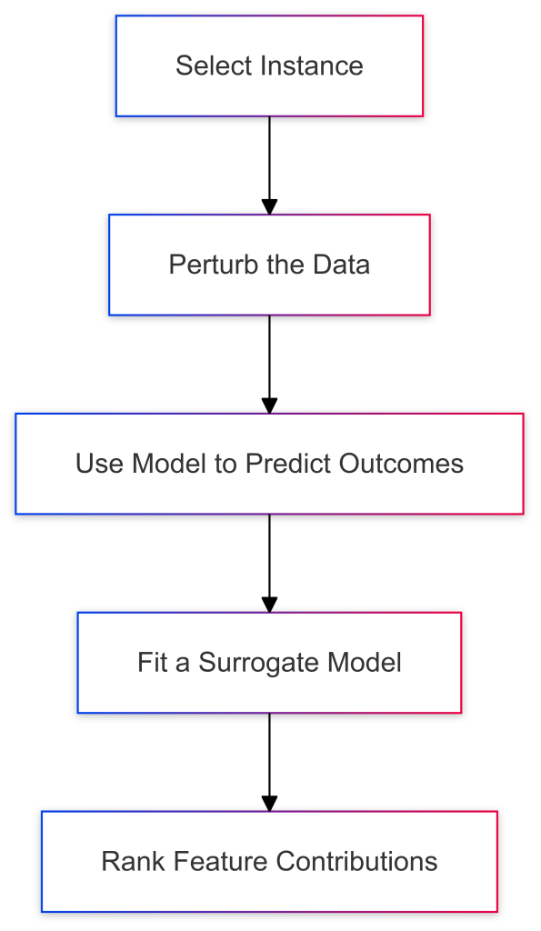
LIME explains a model’s prediction for a specific data point by:
- Perturbing the Instance: Generating synthetic data by slightly modifying the original instance.
- Predicting with the Original Model: Using the trained model to predict outcomes for the perturbed data.
- Fitting a Surrogate Model: Fitting a simpler, interpretable model (e.g., linear regression) to approximate the complex model’s behavior around the instance.
- Ranking Feature Contributions: Determining which features most influenced the prediction.
Visualizing LIME’s Workflow

3. Step-by-Step Implementation
Here’s how to implement LIME on the loan approval model.
3.1 Loading the Pretrained Model and Test Data
Sub-Steps:
- Load the Preprocessed Data:
- Load the Pretrained Model:
3.2 Initializing the LIME Explainer
Sub-Steps:
- Import LIME:
- Initialize the Explainer:
💡 Pro Tip: Ensure all features in training_data are numerical and preprocessed. Missing or unscaled data can lead to incorrect explanations.
3.3 Generating Explanations for Specific Predictions
Sub-Steps:
- Select an Instance:
- Generate the Explanation:
- Inspect the Explanation:
3.4 Visualizing and Interpreting Results
Sub-Steps:
- Display the Explanation in a Notebook:
- Save the Explanation:
- Visualize Feature Contributions:
Output:
4. Real-World Example: Interpreting Loan Approvals
💡 Let’s step into the shoes of John, a loan applicant.
John recently applied for a loan and was denied. Here are the details of his application:
| Feature | Value |
|---|---|
| ApplicantIncome | $2,500 |
| LoanAmount | $200,000 |
| Credit_History | Poor |
🤔 Why Was John’s Application Denied?
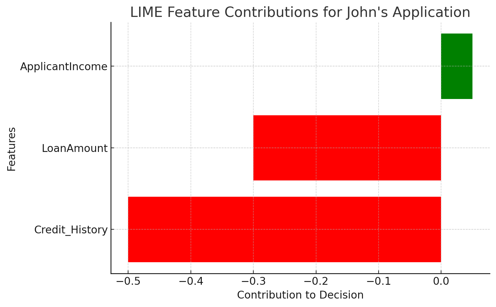
LIME breaks down the decision for John’s application into feature contributions:
| Feature | Contribution | Interpretation |
|---|---|---|
| Credit_History | -0.50 | Poor credit history strongly reduces approval. |
| LoanAmount | -0.30 | High loan amount decreases approval likelihood. |
| ApplicantIncome | +0.05 | Moderate income slightly improves approval odds. |
📊 Visualizing the Explanation:

🔎 Key Insight:
From the explanation:
- Credit History (-0.50): The single most significant factor in denial, due to poor credit history.
- Loan Amount (-0.30): A high loan request further reduced John’s approval chances.
- Applicant Income (+0.05): Slightly improved the odds but was insufficient to offset the negatives.
📈 Compare John’s Case with Another Applicant
To understand John’s situation better, let’s compare his application with an approved applicant:
| Feature | Contribution (John) | Contribution (Approved Applicant) |
|---|---|---|
| Credit_History | -0.50 | +0.70 |
| LoanAmount | -0.30 | -0.10 |
| ApplicantIncome | +0.05 | +0.20 |
Visualization:
- In the approved applicant’s case, Credit_History had a positive contribution (+0.70), significantly increasing their approval odds.
- Their LoanAmount was lower, reducing the negative impact compared to John’s.
- ApplicantIncome contributed more positively, further strengthening their application.
🤔 Does John’s Rejection Seem Justified?
While John’s rejection aligns with the model’s logic, it also raises questions about fairness:
- Should Credit_History dominate decisions this heavily?
- Could LoanAmount be offset by higher income in future iterations of the model?
These insights can guide both applicants and model developers to refine decision criteria for better fairness and transparency.
5. Common Pitfalls and How to Avoid Them
- Improper Data Preprocessing:
Ensure that all features are scaled and numerical before using LIME. - Choosing the Wrong Instance:
Select meaningful instances to explain (e.g., outliers or cases of interest). - Interpreting LIME’s Surrogate Model Globally:
LIME explanations are local and only valid for the specific instance.
6. Key Insights and Takeaways
- Transparency: LIME breaks down predictions into understandable components.
- Trust: By explaining decisions, LIME builds confidence among stakeholders.
- Fairness: Insights from LIME can reveal potential biases in the model.
🔜 What’s Next in This Series?
In Part 4, we’ll:
- Dive into SHAP for understanding both global and local feature contributions.
- Visualize feature interactions and their effects on predictions.
- Address model biases with actionable insights.
Stay tuned as we continue to demystify AI and make it transparent and trustworthy! 🚀

